8 - Chapman MATLAB Programming for Engineers

>>syms s

>>H = s^2 +6*s + 8;

>>G = -H/3

G = -1/3*s^2-2*s-8/3

The result is G = −(1/3)s2 − 2s − 8/3, while we would prefer G = −(s2 + 6s + 8)/3.

13.2Manipulating Trigonometric Expressions

Trigonometric expressions can also be manipulated symbolically in Matlab, primarily with the use of the expand function. For example:

>>syms theta phi

>>A = sin(theta + phi) A =

sin(theta+phi)

>>A = expand(A)

A = sin(theta)*cos(phi)+cos(theta)*sin(phi)

>>B = cos(2*theta) B =

cos(2*theta)

>>B = expand(B)

B = 2*cos(theta)^2-1

>>C = 6*((sin(theta))^2 + (cos(theta))^2) C =

6*sin(theta)^2+6*cos(theta)^2

>>C = expand(C)

C = 6*sin(theta)^2+6*cos(theta)^2

Thus, Matlab was able to apply trigonometric identities to expressions A and B, but it was not successful with C, as we know

C = 6(sin2(θ) + cos2(θ)) = 6

Matlab can also manipulate expressions involving complex exponential functions. For example:

>>syms theta real

>>A = real(exp(j*theta))

A = 1/2*exp(i*theta)+1/2*exp(-i*theta)

257

>> A = simplify(A)

A = cos(theta)

13.3Evaluating and Plotting Symbolic Expressions

In many applications, we eventually want to obtain numerical results or a plot from a symbolic expression. The function double produces numerical results:

double(S) Converts the symbolic matrix expression S to a matrix of double precision floating point numbers. S must not contain any symbolic variables, except possibly eps.

Since the symbolic expression cannot contain any symbolic variables, it is necessary to use subs to substitute numerical values for the symbolic variables prior to applying double. For example:

>>E = s^3 -14*s^2 +65*s -100;

>>F = subs(E,s,7.1)

F = 13671/1000

>> G = double(F) G =

13.6710

The symbolic form is F and the numeric quantity is G, as confirmed by the display from whos:

Grand total is 34 elements using 440 bytes

Symbolic expressions can be plotted with the Matlab function ezplot:

258

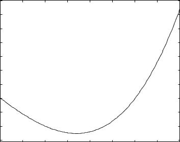
For example consider plotting the polynomial function

A(s) = s3 + 4s2 − 7s − 10

over the range [−1, 3]:

syms s

a = [1 4 -7 -10]; A = poly2sym(a,s)

ezplot(A,-1,3), ylabel(’A(s)’)

The resulting plot is shown in Figure 13.3. Note that the expression plotted is automatically placed at the top of the plot and that the axis label for the independent variable is automatically placed. A ylabel command was used to label the dependent variable.

Figure 13.1: Plot of a polynomial function using ezplot

13.4Solving Algebraic and Transcendental Equations

The symbolic math toolbox can be used to solve algebraic and transcendental equations, as well as systems of such equations. A transcendental equation is one that contains one or more transcendental functions, such as cos x, ex, or ln x.

The function used in solving these equations is solve. There are several forms of solve, but only the following forms will be presented in these notes:

259

solve(E1, E2,...,EN)

solve(E1, E2,...,EN, var1, var2,...,varN)

where E1, E2,...,EN are the names of symbolic expressions and var1, var2,..., varN are variables in the expressions that have been declared to be symbolic. The solutions obtained are the roots of the expressions; that is, symbolic expressions for the variables under the conditions E1 = 0, E2 = 0, . . . EN = 0.

For one equation and one variable, the resulting output solution is returned as a single symbolic variable.

For example:

>>syms s

>>E = s+2;

>>s = solve(E)

s = -2

For N equations, the N solutions are returned as a symbolic vector.

For example:

>>syms s

>>D = s^2 +6*s +9;

>>s = solve(D)

s = [ -3] [ -3]

Thus, the solution is the symbolic representation of the repeated real roots of the quadratic polynomial, providing the same results as those obtained earlier in numeric representation using the function roots. Complex roots can also be obtained, as shown in the following example:

>>syms s

>>P = s^3 -2*s^2 -3*s + 10;

>>s = solve(P)

s =

[ -2] [ 2+i] [ 2-i]

Similar results can be obtained in the solution of transcendental equations. An example in trigonometry:

>> syms theta x z

260

>>E = z*cos(theta) - x;

>>theta = solve(E,theta) theta =

acos(x/z)

For an example involving ex, consider the solution to e2x + 4ex = 32:

>>syms x

>>E = exp(2*x) + 4*exp(x) -32;

>>x = solve(E)

x =

[ log(-8)] [ log(4)]

>>log(-8) ans =

2.0794+ 3.1416i

>>log(4)

ans = 1.3863

Note that two solutions are provided, with the numeric results showing that the first solution log(−8) = 2.0794 + 3.1416i is complex, while the second solution log(4) = 1.3863 is real. The issue as to whether both of these solutions are meaningful would depend on the application that led to the original equation.

Equations containing periodic functions can have an infinite number of solutions. In such cases, solve restricts the search for solutions to the region near 0. For example, to solve the equation cos(2θ) − sin(θ) = 0:

>>E = cos(2*theta)-sin(theta);

>>solve(E)

ans =

[ -1/2*pi] [ 1/6*pi]

[5/6*pi]

Example 13.1 Positioning a robot arm

Consider again the application to robot motion that was presented in Section 10.4. The robot arm has two joints and two links. The (x, y) coordinates of the hand are given by

x1 = L1 cos θ1 + L2 cos(θ1 + θ2)

x2 = L1 sin θ1 + L2 sin(θ1 + θ2)

261

where θ1 and θ2 are the joint angles and L1 = 4 feet and L2 = 3 feet are the link lengths. A part of the previous solution that was not determined was the joint angles needed to position the hand at a given set of coordinates. For the initial hand position of (x, y) = (6.5, 0), the following commands determine the required angles:

>>syms theta1 theta2

>>E1 = 4*cos(theta1)+3*cos(theta1+theta2)-6.5;

>>E2 = 4*sin(theta1)+3*sin(theta1+theta2);

>>[theta1, theta2] = solve(E1,E2)

theta1 =

[ atan(9/197*55^(1/2))] [ atan(-9/197*55^(1/2))]

theta2 =

[ -atan(3/23*55^(1/2))] [ -atan(-3/23*55^(1/2))]

>>theta1 = double(theta1*(180/pi)) theta1 =

18.7170 -18.7170

>>theta2 = double(theta2*(180/pi)) theta2 =

-44.0486 44.0486

There are two solutions, given first in symbolic form, then converted into numeric form using double. The first is θ1 = 18.717◦, θ2 = −44.0486◦, which is the “elbow up” solution. The second is θ1 = −18.717◦, θ2 = 44.0486◦, the “elbow down” solution.

13.5Calculus

Symbolic expressions can be di erentiated and integrated to obtain closed form results.

Di erentiation

The diff function, when applied to a symbolic expression, provides a symbolic derivative.

diff(E) Di erentiates a symbolic expression E with respect to its free variable as determined by findsym.

diff(E,v) Di erentiates E with respect to symbolic variable v.

diff(E,n) Di erentiates E n times for positive integer n.

diff(S,v,n) Di erentiates E n times with respect to symbolic variable v.

262

Examples of derivatives of polynomial functions:

>>syms s n

>>p = s^3 + 4*s^2 -7*s -10;

>>d = diff(p)

d = 3*s^2+8*s-7

>>e = diff(p,2)

e = 6*s+8

>>f = diff(p,3)

f = 6

>>g = s^n;

>>h = diff(g)

h = s^n*n/s

>>h = simplify(h)

h = s^(n-1)*n

Examples of derivatives of transcendental functions:

>>syms x

>>f1 = log(x);

>>df1 = diff(f1) df1 =

1/x

>>f2 = (cos(x))^2;

>>df2 = diff(f2) df2 = -2*cos(x)*sin(x)

>>f3 = sin(x^2);

>>df3 = diff(f3) df3 = 2*cos(x^2)*x

>>df3 = simplify(df3) df3 =

2*cos(x^2)*x

>>f4 = cos(2*x);

>>df4 = diff(f4)

df4 = -2*sin(2*x)

>>f5 = exp(-(x^2)/2);

>>df5 = diff(f5)

df5 = -x*exp(-1/2*x^2)

263

Min-Max Problems

The derivative can be used to find the maximum or minimum of a continuous function, say, f(x), over an interval a ≤ x ≤ b. A local maximum or local minimum (one that does not occur at one of the boundaries x = a or x = b) can occur only at a critical point, which is a point where either df/dx = 0 or df/dx does not exist.

Example 13.2 Minimum cost tank design

Consider again the tank design problem that was solved numerically in Example 7.1. In this problem, the tank radius is R, the height is H and the tank volume is such that

500 = πR2H + 23πR3

The cost of the tank, a function of surface area, is

C = 300(2πRH) + 400(2πR2)

The problem is to solve for R and H providing the minimum cost tank providing the specified volume. The symbolic approach is to solve the volume equation for H as a function of R, express cost C symbolically, then di erentiate C with respect to R and solve the resulting equation for R.

[ -5/2/pi*3^(1/3)*(pi^2)^(1/3)+5/2*i*3^(5/6)/pi*(pi^2)^(1/3)] [ -5/2/pi*3^(1/3)*(pi^2)^(1/3)-5/2*i*3^(5/6)/pi*(pi^2)^(1/3)]

>>Rmins = double(Rmins) Rmin =

4.9237

-2.4619+ 4.2641i -2.4619- 4.2641i

>>Rmin = Rmins(1)

Rmin =

4.9237

264

>>Hmin = double(subs(H,R,Rmin)) Hmin =

3.2825

>>Cmin = double(subs(C,{R,H},{Rmin,Hmin})) Cmin =

9.1394e+004

Note that there are three symbolic solutions for R to provide minimum cost (Rmins). Converting these solutions to numeric quantities with double, we see that the second and third solutions are complex, which are not physically meaningful. Thus, we choose Rmin to be Rmins(1) and we compute Hmin and Cmin from this value. These symbolic results obtained here are more accurate than those determined previously in Example 7.1, as there has been no need to consider samples of R and H at a limited resolution. However, note that the results determined by the two methods are very close.

Integration

The int function, when applied to a symbolic expression, provides a symbolic integration.

Examples of integrals of polynomials:

>>syms x n a b t

>>int(x^n)

ans = x^(n+1)/(n+1)

>>int(x^3 +4*x^2 + 7*x + 10) ans = 1/4*x^4+4/3*x^3+7/2*x^2+10*x

>>int(x,1,t)

ans = 1/2*t^2-1/2

>> int(x^3,a,b) ans = 1/4*b^4-1/4*a^4

Examples of integrals of transcendental functions:

265

>>syms x

>>int(1/x) ans = log(x)

>>int(cos(x)) ans =

sin(x)

>>int(1/(1+x^2)) ans =

atan(x)

>>int(exp(-x^2)) ans = 1/2*pi^(1/2)*erf(x)

The last integral above introduces the error function erf(x) for each element of x, where x is real. The error function is defined as:

erf(x) = 2 x e−t2 dt

√π 0

13.6Linear Algebra

Operations on symbolic matrices can be performed in much the same way as with numeric matrices.

The following are examples of matrix inverse, product, and determinant.

>>A = sym([2,1; 4,3])

A =

[ 2, 1] [ 4, 3]

>>Ainv = inv(A)

Ainv =

[3/2, -1/2]

[ -2, 1]

>>C = A*Ainv

C =

[ 1, 0] [ 0, 1]

>>B = sym([1 3 0; -1 5 2; 1 2 1])

B =

detB = 10

266