

8 - Chapman MATLAB Programming for Engineers
.pdf-2 kmin = 2
The maximum value is found to be 5, the minimum value −2, and the index of the minimum value is 2. Thus, vmin = v(kmin) = v(2) = -2.
For the random data vectors data1 and data2:
>>max(data1) ans =
3.9985
>>min(data1) ans =
2.0005
>>[max2,kmax2] = max(data2) max2 =
5.7316 kmax2 =
256
>>[min2,kmin2] = min(data2) min2 =
0.3558 kmin2 =
268
These results can be approximately confirmed from Figure 7.1.
For a matrix, the min and max functions return a row vector of the minimum or maximum elements of each column of the matrix.
>> B = [-1 1 7 0; -3 5 5 8; 1 4 4 -8] B =
-1 |
1 |
7 |
0 |
-3 |
5 |
5 |
8 |
1 |
4 |
4 |
-8 |
>> min(B) |
|
|
|
ans = |
|
|
|
-3 |
1 |
4 |
-8 |
>> max(B) |
|
|
|
ans = |
|
|
|
1 |
5 |
7 |
8 |
Example 7.1 Minimum cost tank design
A cylindrical tank with a hemispherical top, as shown in Figure 7.2, is to be constructed that will hold 5.00 × 10⁵L when filled. Determine the tank radius R and height H to minimize the tank
137
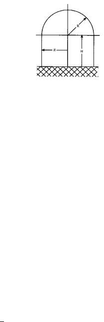
cost if the cylindrical portion costs $300/m2 of surface area and the hemispherical portion costs $400/m2.
Figure 7.2: Tank configuration
Mathematical model:
Cylinder volume: Vc = πR2H
Hemisphere volume: Vh = 23 πR3
Cylinder surface area: Ac = 2πRH
Hemisphere surface area: Ah = 2πR2
Assumptions:
Tank contains no dead air space.
Concrete slab with hermetic seal is provided for the base.
Cost of the base does not change appreciably with tank dimensions.
Computational method:
Express total volume in meters cubed (note: 1m3 = 1000L) as a function of height and radius
Vtank = Vc + Vh
For Vtank = 5 × 10⁵L = 500m3:
500 = πR2H + 23πR3
Solving for H: |
|
|
|
H = |
500 |
− |
2R |
|
|
||
πR2 |
3 |
Express cost in dollars as a function of height and radius
C = 300Ac + 400Ah = 300(2πRH) + 400(2πR2)
138
Method: compute H and then C for a range of values of R, then find the minimum value of C and the corresponding values of R and H.
To determine the range of R to investigate, make an approximation by assuming that H = R. Then from the tank volume:
Vtank = 500 = πR3 + 23πR3 = 53πR3
Solving for R:
R = 300
π
1
3
From Matlab:
>> Rest = (300/pi)^(1/3) Rest =
4.5708
We will investigate R in the range 3.0 to 7.0 meters.
Computational implementation:
Matlab script to determine the minimum cost design:
%Tank design problem
%Compute H & C as functions of R R = 3:0.001:7.0;
H = 500./(pi*R.^2) - 2*R/3;
C = 300*2*pi*R.*H + 400*2*pi*R.^2;
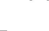
%Plot cost vs radius plot(R,C),title(’Tank Design’),...
xlabel(’Radius R, m’),...
ylabel(’Cost C, Dollars’),grid
%Generate trial radius values R
%Height H
%Cost
% Compute and display minimum cost, corresponding H & R [Cmin kmin] = min(C);
disp(’Minimum cost (dollars):’) disp(Cmin)
disp(’Radius R for minimum cost (m):’) disp(R(kmin))
disp(’Height H for minimum cost (m):’) disp(H(kmin))
139
Running the script:
Minimum cost (dollars): 9.1394e+004
Radius R for minimum cost (m): 4.9240
Height H for minimum cost (m): 3.2816
Note that the radius corresponding to minimum cost (Rmin = 4.9240 is close to the approximate value, Rest = 4.5708 that we computed to assist in the selection of a range of R to investigate. The plot of cost C versus radius R is shown in Figure 7.3.
|
x 10 |
5 |
|
|
Tank Design |
|
|
|
|
|
1.15 |
|
|
|
|
|
|
|
|
|
1.1 |
|
|
|
|
|
|
|
|
Cost C, Dollars |
1.05 |
|
|
|
|
|
|
|
|
1 |
|
|
|
|
|
|
|
|
|
|
|
|
|
|
|
|
|
|
|
|
0.95 |
|
|
|
|
|
|
|
|
|
0.9 |
3.5 |
4 |
4.5 |
5 |
5.5 |
6 |
6.5 |
7 |
|
3 |
||||||||
|
|
|
|
|
Radius R, m |
|
|
|
|
Figure 7.3: Tank design problem: cost versus radius
7.2Sums and Products
If x is a vector with N elements denoted x(n), n = 1, 2, . . . , N, then:
• The sum y is the scalar
N
y = x(n) = x(1) + x(2) + · · · + x(N)
n=1
140
• The product y is the scalar
N
y = x(n) = x(1) · x(2) · · · x(N)
n=1
• The cumulative sum y is the vector having elements y(k), k = 1, 2, . . . , N
k
y(k) = x(n) = x(1) + x(2) + · · · + x(k)
n=1
• The cumulative product y is the vector having elements y(k), k = 1, 2, . . . , N
k
y(k) = x(n) = x(1) · x(2) · · · x(k)
n=1
If X is a matrix with M rows and N columns with elements denoted x(m, n), m = 1, 2, . . . , M, n = 1, 2, . . . , N, then
• The column sum y is the vector having elements y(n), n = 1, 2, . . . , N
M
y(n) = x(m, n) = x(1, n) + x(2, n) + · · · + x(M, n)
m=1
• The column product y is the vector having elements y(n), n = 1, 2, . . . , N
M
y(n) = x(m, n) = x(1, n) · x(2, n) · · · x(M, n)
m=1
• The cumulative column sum Y is the matrix with M rows and N columns with elements denoted y(k, n), k = 1, 2, . . . , M, n = 1, 2, . . . , N
k
y(k, n) = x(m, n) = x(1, n) + x(2, n) + · · · + x(k, n)
m=1
• The cumulative column product Y is the matrix with M rows and N columns with elements denoted y(k, n), k = 1, 2, . . . , M, n = 1, 2, . . . , N
k
y(k, n) = x(m, n) = x(1, n) · x(2, n) · · · x(k, n)
m=1
The Matlab functions implementing these mathematical functions are the following.
141

sum(x) Returns the sum of the elements in vector x, or the row vector of the sum of elements of each column in matrix x
prod(x) Returns the product of the elements in vector x, or the row vector of the product of elements of each column in matrix x
cumsum(x) Returns a vector the same size as x containing the cumulative sum of the elements in vector x, or a matrix the same size as x containing cumulative sums of values from the columns of x.
cumprod(x) Returns a vector the same size as x containing the cumulative product of the elements in vector x, or a matrix the same size as x containing cumulative products of values from the columns of x.
Example 7.2 Summation
The following is a summation identity
N |
N(N2+ 1) |
n=1 n = |
This identity can be checked with Matlab, for example, for N = 8:
>>N = 8;
>>n =1:8;
>>S = sum(n)
S =
36
>>N*(N+1)/2 ans =
36
Example 7.3 Factorial
The factorial of n is expressed and defined as
n! = n · (n − 1) · (n − 2) · · · 1
This can be computed as prod(1:n), as in the following examples:
>>nfact = prod(1:4) nfact =
24
>>nfact = prod(1:70) nfact =
1.1979e+100
142

7.3Statistical Analysis
Many engineering measurements have an element of randomness. Statistics is a branch of applied mathematics involving the analysis, interpretation, and presentation of data including some degree of randomness or uncertainty. In descriptive statistics, the important features or properties of a set of data are summarized or described.
Continuous random variable: A variable vector x, whose elements can have any of a continuum of values for each measurement, or observation.
Population: all possible measurements of a random variable
Sample: finite number of measurements. Assume that N measurements have been made of a random variable, denoted as the vector x, with elements x(n), n = 1, . . . , N.
Frequency distribution of a random variable: indicates the relative frequency with which specific values of this random variable occur in the population.
Histogram: frequency distribution of sample data, indicating the frequency with which sample values fall within ranges of values, called bins.
• Range of values: xmin ≤ x ≤ xmax
• Number of bins: m
• Bin width: ∆x = xmax − xmin m
•Histogram value in bin k: N(k), the number of samples with value xmin + (k − 1)∆x ≤ x ≤ xmin + k∆x. This is also known as the absolute frequency.
The Matlab commands for generating and plotting a histogram are;
143
Command |
Description |
N = hist(x) |
Returns the row vector histogram N of the values in x using 10 |
|
bins. If x is matrix, returns a histogram matrix N operating |
|
on the columns of x. |
N = hist(x,m) |
Returns the row vector histogram N of the values in x using |
|
m bins. |
N = hist(x,xc) |
Returns the row vector histogram N of the values in x using |
|
bin centers specified by xc. |
N = histc(x,edges) |
Counts the number of values in vector x that fall between the |
|
elements in the edges vector (which must contain monoton- |
|
ically non-decreasing values). N is a length(edges) vector |
|
containing these counts. N(k) will count the value x(i) if |
|
edges(k) >= x(i) > edges(k+1). The last bin will count |
|
any values of x that match edges(end). Values outside the |
|
values in edges are not counted. Use -inf and inf in edges |
|
to include all non-NaN values. |
[N,xc] = hist(...) |
Also returns the position of the bin centers in xc. |
hist (...) |
Without output arguments produces a histogram bar plot of |
|
the results. |
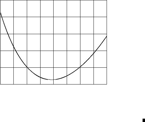
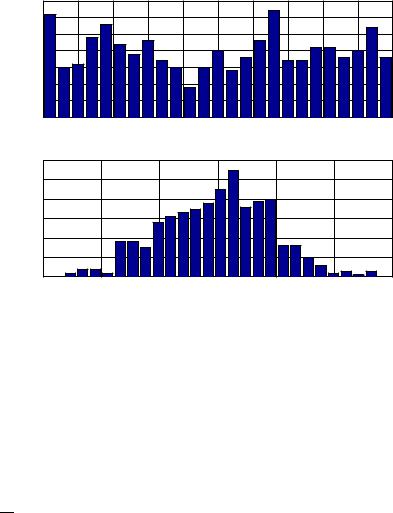
For example, the following commands produce the 25-bin histograms shown in Figure 7.4, operating on the random data vectors data1 and data2.
% Histogram plots
%
subplot(2,1,1),hist(data1,25),...
title(’Histogram of data1’),...
xlabel(’x’),...
ylabel(’N’),...
subplot(2,1,2),hist(data2,25),...
title(’Histogram of data2’),...
xlabel(’x’),...
ylabel(’N’)
Note the di erences in the nature of the two distributions. Random data data1 is called a uniform distribution, as it has roughly equal, or uniform, frequency in all bins. Random data data2 has a bell-shaped distribution, called a Gaussian distribution or Normal distribution.
Relative frequency histogram: The histogram value in bin k is normalized by the total number, N, of data samples: N(k)/N.
The hist function is limited in its ability to produce relative frequency histograms. It is better to generate such plots with the bar function, defined as follows:
144
Histogram of data1
35 |
|
|
|
|
|
|
|
|
|
|
30 |
|
|
|
|
|
|
|
|
|
|
25 |
|
|
|
|
|
|
|
|
|
|
20 |
|
|
|
|
|
|
|
|
|
|
N |
|
|
|
|
|
|
|
|
|
|
15 |
|
|
|
|
|
|
|
|
|
|
10 |
|
|
|
|
|
|
|
|
|
|
5 |
|
|
|
|
|
|
|
|
|
|
0 |
2.2 |
2.4 |
2.6 |
2.8 |
3 |
3.2 |
3.4 |
3.6 |
3.8 |
4 |
2 |
||||||||||
|
|
|
|
|
x |
|
|
|
|
|
Histogram of data2
|
60 |
|
|
|
|
|
|
|
50 |
|
|
|
|
|
|
|
40 |
|
|
|
|
|
|
N |
30 |
|
|
|
|
|
|
|
20 |
|
|
|
|
|
|
|
10 |
|
|
|
|
|
|
|
0 |
1 |
2 |
3 |
4 |
5 |
6 |
|
0 |
||||||
|
|
|
|
x |
|
|
|
Figure 7.4: Absolute frequency histograms
bar(X,Y) |
Draws the columns of the M-by-N matrix Y as M groups of N vertical |
|
bars. The vector X must be monotonically increasing or decreasing. |
bar(Y) |
Uses the default value of X=1:M. |
bar(x,y |
For vector inputs, length(y) bars are drawn, with each bar centered |
|
on a value of x. |
bar(X,Y,width) |
Specifies the width of the bars. Values of width ¿ 1 produce over- |
|
lapped bars. The default value is width=0.8 |
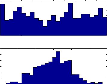
For example, the following commands produce relative histogram plots shown in Figure 7.5 for the random data vectors data1 and data2.
% Relative frequency histogram plots
%
n1 = length(data1); [freq1,x1] = hist(data1,25); rfreq1 = freq1/n1;
n2 = length(data2); [freq2,x2] = hist(data2,25); rfreq2 = freq2/n2;
subplot(2,1,1),bar(x1,rfreq1),...
title(’Relative histogram of data1’), grid,...
xlabel(’x’), ylabel(’relative frequency’),...
subplot(2,1,2),bar(x2,rfreq2),...
title(’Relative histogram of data2’), grid,...
xlabel(’x’), ylabel(’relative frequency’)
145
Relative histogram of data1
|
0.07 |
|
|
|
|
|
|
|
|
|
|
|
0.06 |
|
|
|
|
|
|
|
|
|
|
frequency |
0.05 |
|
|
|
|
|
|
|
|
|
|
0.04 |
|
|
|
|
|
|
|
|
|
|
|
|
|
|
|
|
|
|
|
|
|
|
|
relative |
0.03 |
|
|
|
|
|
|
|
|
|
|
0.02 |
|
|
|
|
|
|
|
|
|
|
|
|
0.01 |
|
|
|
|
|
|
|
|
|
|
|
0 |
2.2 |
2.4 |
2.6 |
2.8 |
3 |
3.2 |
3.4 |
3.6 |
3.8 |
4 |
|
2 |
||||||||||
|
|
|
|
|
|
x |
|
|
|
|
|
Relative histogram of data2
|
0.12 |
|
|
|
|
|
|
|
0.1 |
|
|
|
|
|
|
frequency |
0.08 |
|
|
|
|
|
|
0.06 |
|
|
|
|
|
|
|
relative |
0.04 |
|
|
|
|
|
|
|
|
|
|
|
|
|
|
|
0.02 |
|
|
|
|
|
|
|
0 |
1 |
2 |
3 |
4 |
5 |
6 |
|
0 |
||||||
|
|
|
|
x |
|
|
|
Figure 7.5: Relative frequency histograms
Measures of central tendency
The mean and median describe the middle, or center, of the range of the random variable.
The sample mean of vector x having N elements is x¯
N
x¯ = 1 x(m)
N n=1
The population mean µ (mu) is the value of x¯ for an infinite number of measurements, denoted by
µ = lim x¯
N→∞
where the right hand side is read as “the limit of x bar as N approaches infinity.”
Median: Middle value of a set of random samples, sorted by value (rank ordered). If there is an even number of samples, then the median is the average of the two middle sample values.
Command |
Description |
mean(x) |
Returns the sample mean of the elements of the vector x. Returns a row |
|
vector of the sample means of the columns of matrix x. |
median(x) |
Returns the median of the elements of the vector x. Returns a row vector |
|
of the medians of the columns of matrix x. |
sort(x) |
Returns a vector with the values of vector x in ascending order. Returns a |
|
matrix with each column of matrix x in ascending order. |
146