

Excel2010
.pdf16.If you extend the following series two cells down while the first two cells are selected, what are the new dates in the 3rd and 4th rows?
A
1 Friday, October 01, 2004
2Tuesday, October 05, 2004
a.Friday, October 01, 2005 - Tuesday, October 05, 2006
b.Wednesday, October 06, 2004 - Thursday, October 07, 2004
c.Friday, October 09, 2004 - Tuesday, October 13, 2004
d.Saturday, October 09, 2004 - Wednesday, October 13, 2004
17.To copy format of one cell and apply it to another cell you would use:
a.The Copy Format and the Paste Format commands from Home Styles.
b.The Format Painter button in the Home tab.
c.There is no way to copy and apply formatting in Excel—you would have to do it manually.
d.The Copy and Apply Formatting dialog box, which is located under the Home Format tab.
18.If you want to subtract the values in a range from another range, what do you have to use?
a.Shift+Enter
b.Paste Special
c.Entering numbers with fraction
d.F2
Worksheet and Cell Operations |
31 |

Word Search Puzzle
S P A R A B E C A P S S D
P Y H A I J N C H J C E G
R O K B J Y W F E C R D K
E C O L U M N N R L O H U
A L O O V Y T Z X F L K C
D T B O P E R F X X L S X
S S K T R D R D N E I G P
H O R I Z O N T A L N Z V
E F O R M A T T I N G Q S
E Y W F M X W P W C H C J
T P B M V B D C I L A T I
B J O E N O B B I R L L C
G C W N V C B Q P V K O J
Words |
Clues |
|
|
|
|
SCROLLING |
Move on-screen text or images horizontally or vertically so new information appears |
|
on one side of the screen as older information disappears from the other side. |
||
|
||
|
|
|
|
The longest key on the keyboard. |
|
|
|
|
|
The new style toolbar since Office 2007 |
|
|
|
|
|
A font style. |
|
|
|
|
|
The basic unit of a worksheet into in which you enter data. |
|
|
|
|
|
It’s named with numbers and contains 16,384 cells. |
|
|
|
|
|
Instruction. |
|
|
|
|
|
Changing the color or style of text. |
|
|
|
|
|
Something arranged across. |
|
|
|
|
|
A font style. |
|
|
|
|
|
It is named with letters and contains 1,048,576 cells. |
|
|
|
|
|
A program which allows you to enter formulas in table format and then perform |
|
|
calculations or create graphs. |
|
|
|
|
|
Perpendicular to the horizon. Up and down. |
|
|
|
|
|
Made up of sheets. |
|
|
|
|
|
Default extension of an Excel document. |
|
|
|
32 |
Microsoft Excel |

Practice
Use the next Figure for the questions 1 through 4.
1.Height of the rows in the table is 12.75. Change them to 15.
2.As shown in the figure, range B2:E2 is the title of the table. Move this range to the bottom of the table.
3.Delete the 4th and 7th rows at the same time.
4.Add 3 columns between columns D and E.
5.Write numbers using the Fill Series command.
6.Change the active worksheet without using the mouse.
7.Type your name to all cells in the range A1: P20 using the fastest way.
8.As shown in the Figure below, can you turn yellow colored cells to blue at the same time?
9.Can you select all cells using the keyboard?
10.On the Figure right, Copy the cell C4 to C10 and Move the cell C6 to C11.
Worksheet and Cell Operations |
33 |

11. How can you add the records from Table-2 to Table-1 to produce Table-3.
12.Sometimes you need to change the direction of your lists from vertical to horizontal or vice versa. Show how you can change the list in Table 1 as in Table 2.
13.For the figure below, change the column widths of A, C, and E simultaneously. Then, Auto fit all the columns at the same time.


Figure 3.1: Font Group icons
Figure 3.2: Alignment Group icons
FORMATTING YOUR DOCUMENTS
3.1 Formatting Tools
The old formatting toolbar has been integrated with the new Home tab. The Formatting Tools here provide quick access to commonly used formatting actions. When you put your mouse pointer over an icon, it is highlighted and a descriptive tool tip appears.
The following are brief explanations for some common Home Tab Group icons.
 Selects font name size from drop down lists.
 Increase or decrease font size
 Font Styles: Bold, Italic or Underlined
 Borders: Used to add / modify selected cell borders.
Fill Color: Used to change / apply fill color.
Font Color: Used to change / apply font color.
Dialog Box Launcher: Opens the Format cell Dialog box from which you can change all the properties of the selected cells.
Applies vertical cell alignment to the selected range.
Change text direction in the selected range
Wrap text: Without changing the column width, wraps the text from the end of the column to the next row. See Example 3.1 below.
Applies horizontal cell alignment to the selected range.
Decrease and Increase Indent: Changes the start position of the text without changing the left margin.
Merge cells: Merges selected cell as if they are one cell. Or, unmerges them back.
Example 3.1:
a. Before wrap text |
b. After wrap text |
36 |
Microsoft Excel |

Number Format: Choose how the values in a cell are displayed: as a percentage, as a currency, as a date or time, etc.
Quick access to the currency, percentage or comma style formats.
Increase or decrease the number of floating point digits.
Quick access to the Insert cells button
Quick access to the Delete cells button
Some quick format options like: Row height, Organize sheets or Sheet protection
3.2 Using The Format Cells Dialog Box
This section explains changing formats such as number formatting, alignment, font, border, patterns and protection of a range of cells. In most cases, the number formats that are accessible from the Number group on the Home tab are just fine.
Sometimes, however, you want more control over how your values appear. Excel offers great control over number formats through the use of the Format Cells dialog box. For formatting numbers, you need to use the Number tab.
You can bring up the Format Cells dialog box in several ways. Start by selecting the cell or cells that you want to format and then do the following:
Choose Home Number and click the small dialog box launcher icon.
Choose Home Number, click the Number Format drop-down list, and select More Number Formats from the drop-down list.
Right-click on the selected range and choose Format Cells from the popup menu.
Press the Ctrl+1 shortcut key.
3.2.1 Number
Number formatting refers to the process of changing the appearance of values contained in cells. For faster and easier processing purposes, Excel keeps some other types as numbers in the cells.
For example dates are kept in the cells as numbers. Time info is kept as a fractional number. But, with this formatting option, when showing this number, Excel shows us a date or time info. This is called Number Formatting. In the following sections, you see how to use many of Excel’s formatting options to quickly improve the appearance of your worksheets.
Figure 3.3: Number group icons
Figure 3.4: Cells group icons
Figure 3.5: Dialog box launcher
Remember that number formatting effects only the appearance, not the value. Also remember that the formatting is applied to the selected cells. So, you should select the destination cells, before making any formatting change.
Formatting Documents |
37 |

Category: Select the desired format from the Category box. Each item forms a special formatting on the selected cells.
Sample: The next figure shows how the selected number format looks.
Figure 3.6: Formatting date
Preview the selected number formatting
Selected Category
Details of the selected format
More Information 
Figure 3.7: Number Formatting options
The following are the number-format categories, along with some general comments:
General: The default format; it displays numbers as integers, as decimals, or in scientific notation if the value is too wide to fit in the cell.
Number: Enables you to specify the number of decimal places, whether to use a comma to separate thousands, and how to display negative numbers (with a minus sign, in red, in parentheses, or in red and in parentheses). E.g. Instead of 3.141593 you can define 2 decimal places and it only shows 3.14.
Currency: Enables you to specify the number of decimal places, whether to use a currency symbol, and how to display negative numbers (with a minus sign, in red, in parentheses, or in red and in parentheses). This format always uses a comma to separate thousands. E.g. $2,500.00
Accounting: Differs from the Currency format in that the currency symbols always line up vertically.
Date: Enables you to choose from several different date formats: July 28, 2007, 7/28/07, etc.
Time: Enables you to choose from several different time formats: 10:30, 10:30:00 AM, 14:30, etc.
Percentage: Enables you to choose the number of decimal places and always displays a percent sign: 25%
Fraction: Enables you to choose from among nine fraction formats: 6 7/8 which is 6.875
Scientific: Displays numbers in exponential notation (with an E): 2.00E+05 = 200,000; 2.05E+05 = 205,000. You can choose the number of decimal places to display to the left of E.
Text: When applied to a value, causes Excel to treat the value as text (even if it looks like a number).
38 |
Microsoft Excel |

Special: Contains four additional number formats (Zip Code, Zip Code +4, Phone Number, and Social Security Number).
Custom: Enables you to define custom number formats that aren’t included in any other category.
Key Combination Formatting Applied
Ctrl+Shift+~ : General number format (that is AutoFormat)
Ctrl+Shift+$ : Currency format with two decimal places
Ctrl+Shift+% : Percentage format, with no decimal places
Ctrl+Shift+^ : Scientific notation number format, with two decimal places
Ctrl+Shift+# : Date format with the day, month, and year
Ctrl+Shift+@ : Time format with the hour, minute, and AM or PM
Ctrl+Shift+! : Two decimal places, thousands separator, and a hyphen for negative values
Example 3.2: Do you wonder what day of the week you were born?
Solution: Excel will help you;
1.Type your birthday into B2, for example 12/6/1993. Note: Check your system date format when entering the date. If this is not your date format, Excel may treat it as text or something else.
2.Open the Format Cells Dialog box, and then click the Number tab.
3.Select Date then select “Monday, December 06, 1993” from the type box.
4.Click OK.
3.2.2 Alignment
Alignment changes the horizontal or vertical alignment of cell contents, based on options you choose.
Horizontal: Select an option in the horizontal list 1 to change the horizontal alignment of cell contents. Changing the alignment of data does not change the data or the type.
Vertical: |
2 to change the vertical |
alignment of cell contents. |
|
Indent: 3 |
Each |
increment |
the indent box is equivalent to the width of one character. |
If you see in a cell, it usually means that your column width is not enough to show the formatted text.
1
3
2
5
4
Figure |
Alignment Tab |
Formatting Documents |
39 |
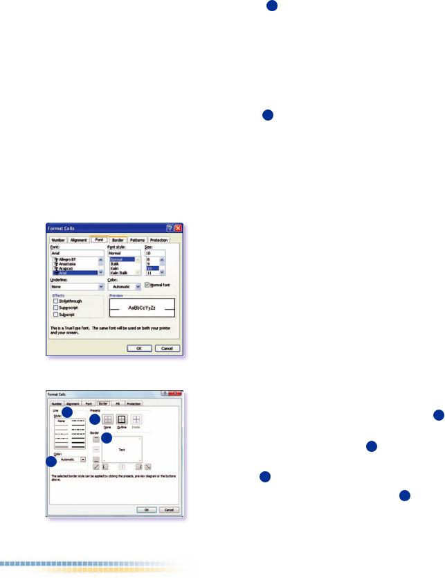
Figure 3.9: Font Tab
3
2
4
Figure .10: Border Tab
Text Control: |
4 You can adjust how you want the text to appear in the cell. |
Wrap Text int |
ultiple lines: The number of wrapped lines depends on the |
width of the column and the length of the cell content. Shrink to fit: If you check this option Excel will automatically reduce the font size so that all data
in the selected |
fits within the column. If you change the column width the |
character size |
adjusted automatically, but the applied font size is not |
changed. Mer |
cells: Joins two or more selected cells into a single cell, or |
unmerges the merged cells. This is often used to create labels that span multiple columns.
Orientation: |
selected cells. |
Degree: You |
enter a number to change text orientation. Use a positive |
number in the |
box to rotate the selected text from bottom left corner |
to upper right |
a negative number in the degree box to rotate the selected |
text from the |
left to the bottom right corner in the cell. |
3.2.3 Font
Font: select |
name to change the font of the selected cell text. |
Font style: select a font style of the selected cell text. |
|
Size: select |
size for the selected cell text. You can type any number |
between 1 |
to change the size. |
Underline: select an underline type format to apply to the selected cell text.
Color: select |
from the list to apply to the selected cell text. |
Effects: select |
to apply from the Effects group box. |
Strikethrough: |
a line through the selected text. |
Superscript: |
the format of the selected text to superscript Eg. x2 |
Subscript: changes the format of the selected text to subscript Eg. H2O
Preview: shows how the selected text will appear.
3.2.4 Borders
Presets: Apply |
border style using the |
1 or remove an old |
border style. |
|
|
Line Style: |
3 , then click |
border to which you |
want to apply the new line style. |
|
|
Line Color: 4 |
|
the line color. |
Border: You |
add/remove any Border lines 2 by clicking on them. The |
|
new lines will have the color and style you selected.
40 |
Microsoft Excel |