

1Foundation of Mathematical Biology / Foundation of Mathematical Biology
.pdfUCSF What happened when we applied the t test naively?
We compute 6817 t-statistics (one for each gene)
What is the critical value?
♦P = 0.05
♦N = 27
♦M = 11
♦Degrees of freedom = 27+11-2 = 36
♦Critical value (two-tailed test): 2.03
Of the 6817 genes, 1636 are “significant”
Less than 40% of these are significant on the test set!
What happened?
We made 6817 independent tests of a statistic at a significance level of 0.05
We should expect about 341 genes to show up even if we have no real effect, assuming that our statistical assumptions are OK
How can we use permutation to do a better job?
UCSF |
Permutation analysis in array data: |
|
Conservative approach is to take the max statistic |
||
|
|
|
We are defining our new statistic to be one computed over the vector of all genes coupled to the class information
We define our statistic to be the maximum of a particular statistic, computed for each gene
We will use two statistics
♦Kendall’s Tau, measuring the rank correlation of gene expression levels against the AML/ALL classes represented as 0 and 1
♦The t statistic, functionally implemented on paired data of gene expression levels and classes represented as 0 and 1
♦For each case, we define our new statistic as the max(over all genes)

UCSF |
|
|
|
|
|
|
Permutation analysis in array data: |
|||||
|
|
Conservative approach is to take the max statistic |
||||||||||
|
Sample |
|
|
|
|
Genes 1…9 |
|
|
|
|
Class |
|
1 |
0.99 |
0.98 |
0.98 |
0.97 |
0.97 |
0.95 |
0.95 |
0.95 |
0.96 |
|
1 |
|
|
||||||||||||
2 |
1.15 |
1.11 |
1.07 |
1.04 |
1.01 |
0.99 |
0.98 |
0.96 |
0.96 |
|
1 |
|
|
||||||||||||
3 |
1.11 |
1.14 |
1.22 |
1.3 |
1.37 |
1.39 |
1.39 |
1.39 |
1.37 |
|
1 |
|
|
||||||||||||
4 |
1 |
1.01 |
1.01 |
0.99 |
0.96 |
0.93 |
0.91 |
0.89 |
0.88 |
|
1 |
|
|
||||||||||||
5 |
1.04 |
1.01 |
0.97 |
0.94 |
0.93 |
0.92 |
0.9 |
0.9 |
0.91 |
|
1 |
|
|
||||||||||||
6 |
1.17 |
1.25 |
1.32 |
1.38 |
1.43 |
1.46 |
1.5 |
1.53 |
1.55 |
|
0 |
|
|
||||||||||||
7 |
1.12 |
1.16 |
1.2 |
1.26 |
1.34 |
1.42 |
1.49 |
1.54 |
1.53 |
|
0 |
|
|
||||||||||||
8 |
0.96 |
0.97 |
0.97 |
0.97 |
0.96 |
0.96 |
0.97 |
0.98 |
0.98 |
|
0 |
|
|
||||||||||||
9 |
1.03 |
1.04 |
1.05 |
1.06 |
1.07 |
1.09 |
1.1 |
1.12 |
1.17 |
|
0 |
|
|
||||||||||||
10 |
1.16 |
1.19 |
1.21 |
1.23 |
1.25 |
1.25 |
1.26 |
1.27 |
1.28 |
|
0 |
|
|
||||||||||||
|
|
0.16 |
0.24 |
0.18 |
0.27 |
0.27 |
0.27 |
0.38 |
0.38 |
0.42 |
|
|
Statistic for each gene
Maximum magnitude statistic

UCSF |
|
|
|
|
|
Permutation 1: Bogus correlation |
|||||
|
Sample |
|
|
|
|
Genes 1…9 |
|
|
|
Class |
|
1 |
0.99 |
0.98 |
0.98 |
0.97 |
0.97 |
0.95 |
0.95 |
0.95 |
0.96 |
1 |
|
2 |
1.15 |
1.11 |
1.07 |
1.04 |
1.01 |
0.99 |
0.98 |
0.96 |
0.96 |
1 |
|
3 |
1.11 |
1.14 |
1.22 |
1.3 |
1.37 |
1.39 |
1.39 |
1.39 |
1.37 |
1 |
|
4 |
1 |
1.01 |
1.01 |
0.99 |
0.96 |
0.93 |
0.91 |
0.89 |
0.88 |
1 |
|
5 |
1.04 |
1.01 |
0.97 |
0.94 |
0.93 |
0.92 |
0.9 |
0.9 |
0.91 |
1 |
|
6 |
1.17 |
1.25 |
1.32 |
1.38 |
1.43 |
1.46 |
1.5 |
1.53 |
1.55 |
0 |
|
7 |
1.12 |
1.16 |
1.2 |
1.26 |
1.34 |
1.42 |
1.49 |
1.54 |
1.53 |
0 |
|
8 |
0.96 |
0.97 |
0.97 |
0.97 |
0.96 |
0.96 |
0.97 |
0.98 |
0.98 |
0 |
|
9 |
1.03 |
1.04 |
1.05 |
1.06 |
1.07 |
1.09 |
1.1 |
1.12 |
1.17 |
0 |
|
10 |
1.16 |
1.19 |
1.21 |
1.23 |
1.25 |
1.25 |
1.26 |
1.27 |
1.28 |
0 |
|
|
|
0.15 |
0.09 |
0.09 |
0.04 |
0.02 |
0.02 |
0.02 |
0.07 |
0.04 |
|
Statistic for each gene
Maximum magnitude statistic
UCSF
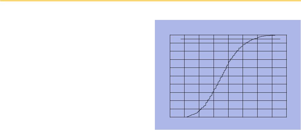
Repeated permutation yields a cumulative distribution
Unadjusted critical value
♦τ = 0.17
♦Yields 1751 genes as “significant”
♦Less than half confirmed on the test set
Adjusted critical value
♦τ = 0.354
♦51 genes significant
♦90% of these are confirmed on the test set
Permutation Based Estimation of Significance
|
1 |
|
|
|
|
|
|
|
|
|
0.9 |
|
|
|
|
|
|
|
|
|
0.8 |
|
|
|
|
|
|
|
|
Proportion |
0.7 |
|
|
|
|
|
|
|
|
0.6 |
|
|
|
|
|
|
|
|
|
0.5 |
|
|
|
|
|
|
|
|
|
Cumulative |
0.4 |
|
|
|
|
|
|
|
|
0.3 |
|
|
|
|
|
|
|
|
|
0.2 |
|
|
|
|
|
|
|
|
|
|
|
|
|
|
|
|
|
|
|
|
0.1 |
|
|
|
|
|
|
|
|
|
0 |
|
|
|
|
|
|
|
|
|
0.24 |
0.26 |
0.28 |
0.3 |
0.32 |
0.34 |
0.36 |
0.38 |
0.4 |
|
|
|
|
|
Max(τ) |
|
|
|
|
From the cumulative distribution, we observe that τ = 0.354 corresponds to p = 0.05.
UCSF |
We get similar results using the T test |
|
|
|
|
Unadjusted critical value
♦t = 2.03
♦Yields 1636 genes as “significant”
♦Less than half confirmed on the test set
Adjusted critical value
♦t = 5.16
♦40 genes significant
♦80% of these are confirmed on the test set
Is it safe to conclude anything about more than just the gene with the max statistic?
♦Yes.
♦If we were to generate the null distribution of the mth best gene, the 95th percentile would be lower than our initial critical value.
Is this estimate better than Bonferonni?
♦It can be.
♦If there are strong cross-correlations in the data, this procedure is not penalized by the redundancy.
♦The Bonferonni correction makes the implicit assumption that all variables are independent.
UCSF
CGH Analysis: Visualization and Correlation with Outcome
Data (J. Gray, K. Chin) |
Is there a statistically significant correlation |
||
♦ 60 CGH profiles |
between CGH profile similarity and outcome |
||
• |
1225 “observables” |
(e.g. survival)? |
|
• |
52 tumor profiles |
|
|
• |
8 normal profiles |
Are there relationships among the measured |
|
♦ Patient information |
|||
variables? |
|||
• |
Age of onset |
||
|
|||
• |
Overall survival |
|
|
• |
Disease free survival |
|
|
• |
Alive or dead |
|
|
|
|
|
|
|
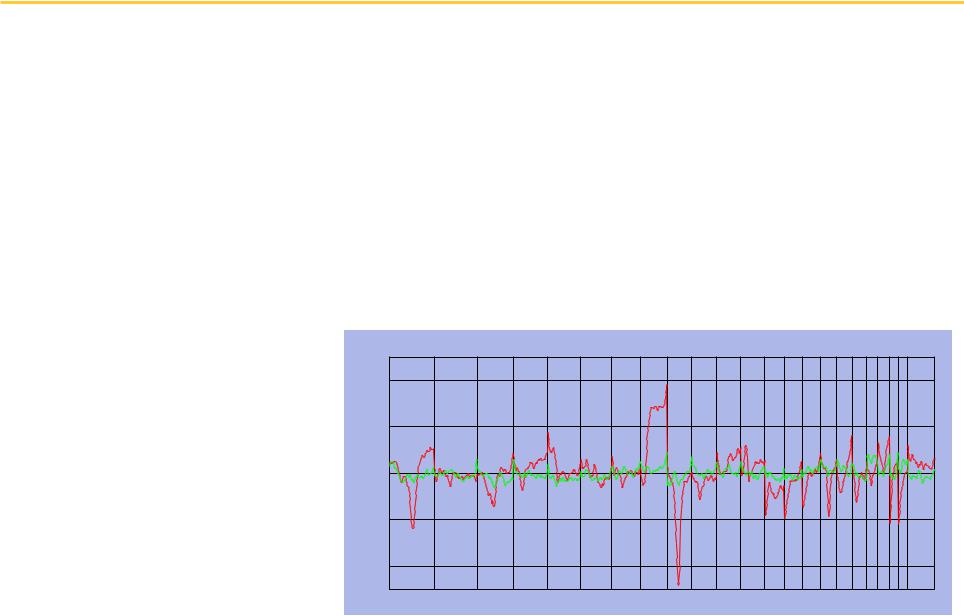
Tumor and Normal CGH Profiles |
|
|
|
|
|
|
|
|
||||
|
|
|
|
|
|
|
|
|
|
|
|
|
|
|
|
|
|
|
|
||
♦ Tumor status |
|
0.4 |
|
|
|
|
|
|
|
|
|
|
|
|
|
|
|
|
|
|
|
|
|
|
|
|
|
|
|
|
|
|
|
|
|
|
|
|
|
|
|
|
|
• |
Size/Stage |
number) |
0.2 |
|
|
|
|
|
|
|
|
|
|
|
|
|
|
|
|
|
|
|
|
|
|
|
|
|
|
|
|
|
|
|
|
|
|
|
|
|
|
||
• |
Estrogen receptor |
|
|
|
|
|
|
|
|
|
|
|
|
|
|
|
|
|
|
|
|
copy |
0 |
|
|
|
|
|
|
|
|
|
|
|
|
|
|
|
|
|
|
||
• |
Progesterone |
|
|
|
|
|
|
|
|
|
|
|
|
|
|
|
|
|
|
||
Log(Relative |
|
|
|
|
|
|
|
|
|
|
|
|
|
|
|
|
|
|
|||
|
|
|
|
|
|
|
|
|
|
|
|
|
|
|
|
|
|
|
|||
|
receptor |
-0.2 |
|
|
|
|
|
|
|
|
|
|
|
|
|
|
|
|
|
|
|
• |
p53 |
|
|
|
|
|
|
|
|
|
|
|
|
|
|
|
|
|
|
|
|
|
|
|
-0.4 |
|
|
|
|
|
|
|
|
|
|
|
|
|
|
|
|
|
|
|
|
|
1 |
2 |
3 |
4 |
5 |
6 |
7 |
8 |
9 |
10 |
11 |
12 |
13 |
14 |
15 |
16 |
17 |
18 |
19 20 2122 X |
|
|
|
|
|
|
|
|
|
|
Genomic Position |
|
|
|
|
|
|
|
|
|
||

UCSF |
We can visualize complex profile data |
|
using 3D virtual worlds |
||
|
|
|
S
u r
v i v
a l
Alive
|
|
|
|
|
|
|
|
|
|
|
|
)) |
|
|
|
|
|
|
|
|
|
|
|
|
ll |
|
|
|
|
|
|
|
|
|
|
|
aa |
|
|
|
|
|
|
|
|
|
|
|
mm |
|
|
|
|
|
|
|
|
|
|
|
rr |
|
|
|
|
|
|
|
|
|
|
|
oo |
|
|
|
|
|
|
|
|
|
|
|
nn |
|
|
|
|
|
|
|
|
|
|
|
|
// |
|
|
|
|
|
|
|
|
|
|
|
rr |
|
|
|
|
|
|
|
|
|
|
|
oo |
|
|
|
|
|
|
|
|
|
|
|
mm |
|
|
|
|
|
|
|
|
|
|
|
uu |
|
|
|
|
|
|
|
|
|
|
|
|
tt |
|
|
|
|
|
|
|
|
|
|
|
(( |
|
|
|
|
|
|
|
|
|
|
|
gg |
|
|
|
|
|
|
|
|
|
|
|
oo |
|
|
|
|
|
|
|
|
|
|
|
|
L |
|
|
|
|
|
|
|
|
|
|
|
|
Dead
|
|
|
|
|
|
|
|
|
|
n |
|
|
|
|
|
|
|
|
|
io |
|
|
|
|
|
|
|
|
|
|
t |
|
|
|
|
|
|
|
|
|
a |
|
|
|
|
|
|
|
|
|
c |
|
|
|
|
|
|
|
|
|
o |
|
|
|
|
|
|
|
|
|
l |
|
|
|
|
|
|
|
|
|
e |
|
|
|
|
|
|
|
|
|
m |
|
|
|
|
|
|
|
|
|
o |
|
|
|
|
|
|
|
|
|
n |
|
|
|
|
|
|
|
|
|
e |
|
|
|
|
|
|
|
|
|
|
G |
|
|
|
|
|
|
|
|
|
|

UCSF |
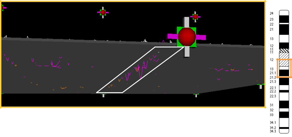
By sliding the opaque XZ plane, |
|
we can select peaks above background |
||
|
|
|
Normals shown in white at survival = -1 month
One remaining background peak from normals
UCSF |
One particular locus sticks out |
|
|
|
|
CHR 9
♦The center of this valley is on chromosome 9
♦The normal profiles show a slight depression there as well
♦Is this locus significant?