

1Foundation of Mathematical Biology / Foundation of Mathematical Biology
.pdfUCSF |
Testing a mean when SD not known |
|
|
|
|
Process is very similar to confidence intervals.
We want to test whether our mean is different from a particular value.
Compute t as follows:
t = (X − 0 ) s
 n
n
For a particular level α and n-1 degrees of freedom, we look up t for 2 α

UCSF
Test of the difference of two sample means: T-test with equal variances
Two samples of size n and m, with sample SD U and V and sample means X and Y:
t =
X −Y
S  1n + m1
|
|
S = |
(n −1)U + (m −1)V |
|
n + m − 2 |
We use n+m-2 as the number of degrees of freedom in finding our critical value.

UCSF
Expression array example: Lymphoblastic versus myeloid leukemia
Lander data
♦6817 unique genes
♦Acute Lymphoblastic Leukemia and Acute Myeloid Leukemia (ALL and AML) samples
♦RNA quantified by Affymax oligo-technology
♦38 training cases (27 ALL, 11 AML)
♦34 testing cases (20/14)
We will consider whether any of the genes are differently expressed between the ALL and
AML classes
R E P O R T S
Molecular Classification of
Cancer: Class Discovery and
Class Prediction by Gene
Expression Monitoring
T.R. Golub,1,2*† D. K. Slonim,1† P. Tamayo,1 C. Huard,1 M. Gaasenbeek,1 J. P. Mesirov,1 H. Coller,1 M. L. Loh,2
J. R. Downing,3 M. A. Caligiuri,4 C. D. Bloomfield,4
E.S. Lander1,5*
Although cancer classification has improved over the past 30 years, there has been no general approach for identifying new cancer classes (class discovery) or for assigning tumors to known classes (class prediction). Here, a generic approach to cancer classification based on gene expression monitoring by DNA microarrays is described and applied to human acute leukemias as a test case. A class discovery procedure automatically discovered the distinction between acute myeloid leukemia (AML) and acute lymphoblastic leukemia (ALL) without previous knowledge of these classes. An automatically derived class predictor was able to determine the class of new leukemia cases. The results demonstrate the feasibility of cancer classification based solely on gene expression monitoring and suggest a general strategy for discovering and predicting cancer classes for other types of cancer, independent of previous biological knowledge.
SCIENCE VOL 286 15 OCTOBER 1999

UCSF
We have two classes: Use the T-statistic
We compute 6817 t-statistics (one for each gene)
What is the critical value?
♦P = 0.05
♦N = 27
♦M = 11
♦Degrees of freedom = 27+11-2 = 36
♦Critical value (two-tailed test): 2.03
Of the 6817 genes, 1636 are “significant”
Less than 40% of these are significant on the test set!
What happened?
We made 6817 independent tests of a statistic at a significance level of 0.05
We should expect about 341 genes to show up even if we have no real effect
We can correct for this in many ways. One is to use a critical value for 0.05/6817 (due to Bonferonni).
We will talk about other methods to avoid these problems in the next lecture

UCSF |
Frequency distribution of sample variance |
|
|
|
|
We discussed the frequency distribution of sample means The Chi-square distribution is also important
If Xi are drawn from a normal distribution with variance σ2, the following distribution will follow Chi-square
(n −1)s2
σ 2
We can derive confidence intervals on sample variances as we did with sample means.
More important, however, are the Chi-squared tests for goodness of fit and Chi-squared tests in contingency tables.
UCSF |
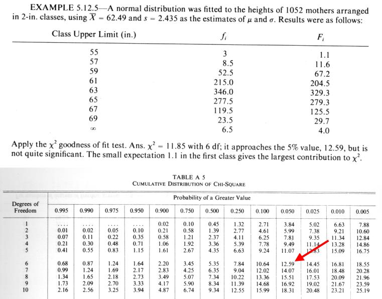
Chi-squared test of goodness of fit |
|
|
|
|
We have some hypothesis about the true distribution from which a set of observations were drawn
We compute the following value:
k |
( f |
i |
− F )2 |
χ 2 = ∑ |
|
i |
|
|
|
Fi |
|
i=1 |
|
|
We use (k-1) for the number of degrees of freedom.
If we had to estimate values for the parent distribution, we reduce the number of degrees of freedom (e.g. (k-3) if we estimated the mean and SD from the data)
UCSF |
Example: Chi-squared test of goodness of fit |
|
|
|
|
UCSF |
Contingency tables |
|
|
|
|
Very often, we have data where each sample is classified by two different characteristics into disjoint subsets
Example: Set of patients in a study
♦Treatment group versus control group
♦Responders versus non-responders
We can use RxC contingency tables to decide whether there is any significance difference among the groups in terms of deviations from expected frequencies.
UCSF |
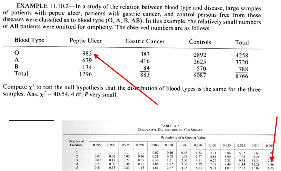
Chi-square example: RxC table |
|
|
|
|
( f − F )2
∑ F
F = (1796/8766)*(4258/8766)*8766 = 872.4 DF = (R-1)(C-1) = 4
UCSF |
What about paired data? |
|
|
|
|
Thus far, we have considered the comparison of unpaired data.
The most common parametric method for considering paired data is
Pearson’s correlation, r
n |
|
|
|
|
|
|
|
|
|
|
( Xi − Xi )(Yi −Yi ) |
||||||||||
r = ∑ |
||||||||||
|
|
|
|
|
|
|
|
|
||
(∑( Xi − Xi )2 )(∑(Yi −Yi )2 ) |
||||||||||
i=1 |
||||||||||
R ranges from -1 to 1. It is exactly 1 if X and Y are linearly related with positive slope. It is exactly -1 is X and Y are linearly related with negative slope.
It is extremely sensitive to outliers.
We will discuss non-parametric methods to deal with paired data in the next lecture. Mark Segal will talk about regression.