

1Foundation of Mathematical Biology / Foundation of Mathematical Biology
.pdfUCSF
Example: Uniform discrete distribution (0…100)
k |
100 |
1 |
|
|
1 |
|
100(100 +1) |
|
||||
µ = ∑Pj X j = ∑ |
|
|
|
X = |
|
|
|
|
|
= 50 |
||
101 |
101 |
2 |
||||||||||
j=1 |
X =0 |
|
|
|||||||||
σ = |
k |
P (X |
j |
− µ )2 |
= |
101 |
1 (X − 50)2 |
= 29.155 |
|
∑ j |
|
|
∑ |
101 |
|
||
|
j=1 |
|
|
|
|
X =0 |
|
|
|
|
|
|
|
n |
|
n |
|||
|
|
|
|
|
∑Xi |
|
∑(Xi − |
|
)2 |
|
|
|
|
( X1 + X 2 +m+ X n ) |
|
|
X |
||||
|
|
|
|
i 1 |
s = |
i=1 |
||||
|
|
|
|
|||||||
X = |
|
= |
= |
n −1 |
||||||
n |
n |
|||||||||
|
|
|
|
|
||||||

UCSF
Consider the sample mean of this uniform distribution
The parent distribution is uniform, with mean 50 and standard deviation 29.155
What is the distribution of sample means from this parent distribution?
Let’s pick n (= 1, 3, 100) observations, with replacement, from this distribution, and compute the sample mean many times (100,000)
♦What will the mean of the sample means be?
♦What will the standard deviation of the sample means be?
♦What will the distribution of the sample means look like?
UCSF |
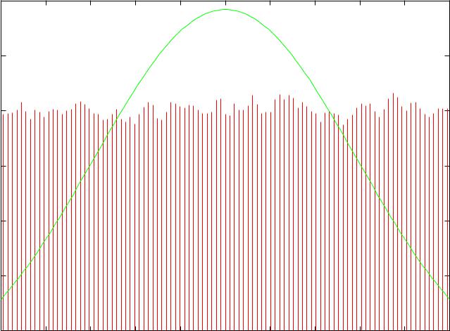
N = 1: We see a uniform distribution |
|
|
|
|
0.014 |
|
|
|
|
|
|
|
|
|
|
0.012 |
|
|
|
|
|
|
|
|
|
|
0.01 |
|
|
|
|
|
|
|
|
|
|
0.008 |
|
|
|
|
|
|
|
|
|
|
0.006 |
|
|
|
|
|
|
|
|
|
|
0.004 |
|
|
|
|
|
|
|
|
|
|
0.002 |
|
|
|
|
|
|
|
|
|
|
0 |
10 |
20 |
30 |
40 |
50 |
60 |
70 |
80 |
90 |
100 |
Mean 50.148270 (pop mean: 50) SD 29.138903 (pop sd: 29.155) |
||||||||||
UCSF |
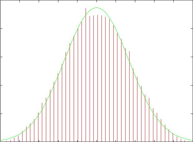
N = 3: Pretty close to normal |
|
|
|
|
0.025 |
|
|
|
|
|
|
|
|
|
|
0.02 |
|
|
|
|
|
|
|
|
|
|
0.015 |
|
|
|
|
|
|
|
|
|
|
0.01 |
|
|
|
|
|
|
|
|
|
|
0.005 |
|
|
|
|
|
|
|
|
|
|
0 |
|
|
|
|
|
|
|
|
|
|
0 |
10 |
20 |
30 |
40 |
50 |
60 |
70 |
80 |
90 |
100 |
Mean 50.089103 (CLT 50) SD 16.785106 (16.8326) |
||||||||||
UCSF |
|
|
|
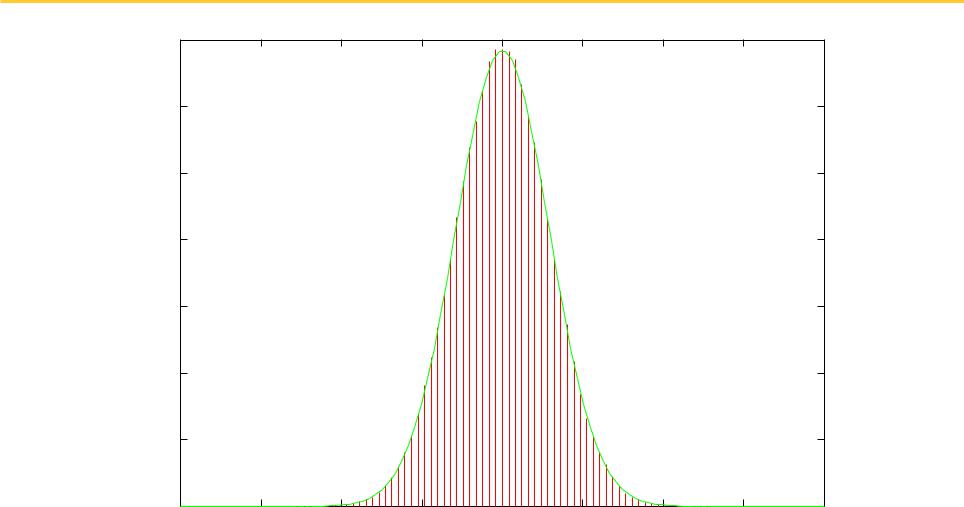
N = 100: Essentially normal |
||||
0.14 |
|
|
|
|
|
|
|
|
0.12 |
|
|
|
|
|
|
|
|
0.1 |
|
|
|
|
|
|
|
|
0.08 |
|
|
|
|
|
|
|
|
0.06 |
|
|
|
|
|
|
|
|
0.04 |
|
|
|
|
|
|
|
|
0.02 |
|
|
|
|
|
|
|
|
0 |
|
|
|
|
|
|
|
|
30 |
35 |
40 |
45 |
50 |
55 |
60 |
65 |
70 |
|
Mean 49.996305 (CLT 50) SD 2.916602 (2.916) |
|
||||||
UCSF |
So now what? |
|
|
|
|
We have a theorem that tells us something about the relationship between the sample mean and the population mean.
We can begin to make statements about what a population mean is likely to be given that we have computed a sample mean.
UCSF
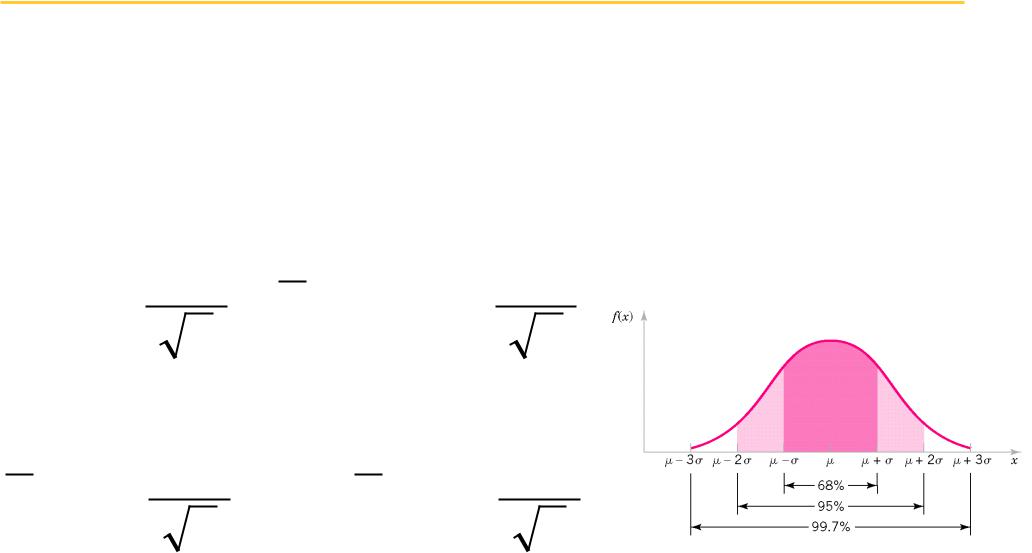
Suppose we know the population standard deviation (this never happens)
We assume that the sample mean computed from n observations comes from a distribution with mean and standard deviation sigmapop/sqrt(n)
So, 95% of the time:
µ −1.96 |
σ pop < X |
< µ +1.96 |
σ pop |
|
n |
|
n |
|
or |
|
|
X −1.96 |
σ pop < µ |
< X +1.96 |
σ pop |
|
n |
|
n |
This is the 95% confidence interval for

UCSF
Suppose we don’t know the population standard deviation (this always happens)
We will use the sample standard deviation s as an estimate for the population standard deviation.
The procedure is very similar to the previous confidence interval, but the distribution follows Student’s t distribution instead of the normal distirbution.
X −1.96 |
σ pop < < X +1.96 |
σ pop |
|
|
n |
|
n |
X − t0.05 |
s < < X + t0.05 |
s |
|
|
n |
n |
|
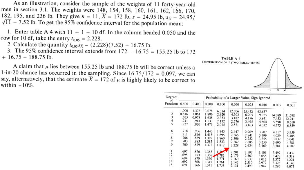
This is the 95% confidence interval for . We look up t in a table that depends on n-1 and 0.05.
UCSF |
Confidence Interval Example |
|
|
|
|
UCSF |
Statistical Hypothesis Testing |
|
|
|
|
We wish to test whether we’ve seen a real effect
♦H0 denotes the null hypothesis: no real effect
♦H1 denotes the alternative: real effect
Statistical jargon
♦Rejecting H0 when it is true is defined as a type I error
•Informally: false positive
•Significance level: probability of rejecting H0 when it is true
♦Rejecting H1 when it is true is a type II error
•Informally: false negative
•Power: probability of rejecting H0 when it is false
When we know the distributions
(or can safely make assumptions) we can use tests like the t-test
When we cannot, we must use non-parametric tests (next lectures)