

Baer M., Billing G.D. (eds.) - The role of degenerate states in chemistry (Adv.Chem.Phys. special issue, Wiley, 2002)
.pdf182 |
|
|
|
|
|
|
satrajit adhikari and gert due billing |
|||||||||
Fx, and so on, we obtain |
|
|
|
|
|
|
|
|
||||||||
|
|
|
|
|
|
|
|
|
Fx ¼ FðX þ x tg f=d12Þ |
ð102Þ |
||||||
|
|
|
|
|
|
|
|
|
Fy ¼ FðY þ y tg f=d12Þ |
ð103Þ |
||||||
|
|
|
|
|
|
|
|
|
Fz ¼ FðZ þ z tg f=d12Þ |
ð104Þ |
||||||
|
|
|
|
|
|
|
|
|
FX ¼ Fðx X tg fd12Þ |
ð105Þ |
||||||
|
|
|
|
|
|
|
|
|
FY ¼ Fðy Y tg fd12Þ |
ð106Þ |
||||||
|
|
|
|
|
|
|
|
|
FZ ¼ Fðz Z tg fd12Þ |
ð107Þ |
||||||
where the |
function F is given as |
F ¼ ðh=2mÞcos f sin f=ðr RÞ and d12 ¼ |
||||||||||||||
m |
1ð |
1 |
|
m |
|
M |
Þ=m |
with M |
¼ |
m |
m |
2 þ |
m |
|
[72,73]. In |
six dimensions, the |
|
|
1 |
= |
|
|
1 þ |
|
|
3 |
|
6 |
|||||
amplitudes diðtÞ [in Eq. (97)] will be of dimension N ¼ i¼1Ni. Here, in mass scaled coordinates we have used [48]
r2=d12 |
¼ |
1 |
r2ð1 |
þ sin y cos fÞ |
||
|
||||||
2 |
||||||
R2d12 |
¼ |
1 |
r2ð1 |
sin y cos fÞ |
||
|
||||||
2 |
||||||
r R ¼ |
1 |
r2sin y sin f |
||||
|
||||||
2 |
||||||
ð108Þ
ð109Þ
ð110Þ
Since the geometric phase effect is related to the angle f we express f as
|
|
tg |
|
r R |
|
|
|
|
|
f ¼ r2=d1 d1R2 |
|
|
|||
|
|
|
|
|
|
||
and obtain |
|
|
|
|
|
|
|
qf |
cos f sin f |
|
2 |
|
|||
|
|
¼ |
|
|
ðX þ x tg f=d1 |
Þ |
|
|
qx |
|
r R |
||||
qf cos f sin f |
2 |
|
|
||||
|
|
¼ |
|
|
ðx X tg fd1 |
Þ |
|
|
qX |
|
r R |
|
|||
ð111Þ
ð112Þ
ð113Þ
plus similar expressions for the y and z components.
Note that in this TDGH–DVR formulation of quantum dynamics, the inclusion of the geometric phase effects through the addition of a vector potential is very simple and the calculations can be carried out with about the same effort as what is involved in the ordinary scattering case.
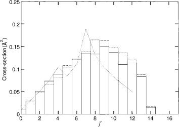
Figure 3 shows the results with and without including the geometric phase effect for the D þ H2 reaction. The basis set is taken as 1,1,1,15,15,15, that is,
non-adiabatic effects in chemical reactions |
183 |
Figure 3. Cross-sections obtained with a (1,1,1,15,15,15) basis set and the TDGH–DVR method for the D þ H2 ðv ¼ 1; j ¼ 1Þ ! DH ðv0 ¼ 1; j0Þ þ H reaction at 1.8-eV total energy. The solid line indicates the values obtained without the vector potential and the dashed with a vector potential. The dashed line indicates the experimental results [49–52].
the X; Y; Z variables are treated classically. Altogether 200 trajectories were calculated. We notice that the branching ration, that is, the total reactive crosssection is obtained from the trajectories but the distribution is obtained by a projection of the DVR points on final rotational–vibrational states of the product. The maximum of the distribution is now j0 ¼ 9 (in better agreement with full quantum calculations). It is shifted to j0 ¼ 8 if the geometric phase is included. The agreement with experimental data is good for j0 values <8 but overestimated at higher values. Since part of the system is still treated classically, we attribute this discrepancy to the lacking ability of classical trajectories to yield proper state-resolved reaction cross-sections (see also Fig. 1).
V.CONCLUSION
In this chapter, we discussed the significance of the GP effect in chemical reactions, that is, the influence of the upper electronic state(s) on the reactive and nonreactive transition probabilities of the ground adiabatic state. In order to include this effect, the ordinary BO equations are extended either by using a HLH phase or by deriving them from first principles. Considering the HLH phase due to the presence of a conical intersection between the ground and the first excited state, the general form of the vector potential, hence the effective
184 |
satrajit adhikari and gert due billing |
kinetic energy operator, for a quasi-JT model and for an A þ B2 type reactive system were presented.
The ordinary BO approximate equations failed to predict the proper symmetry allowed transitions in the quasi-JT model whereas the extended BO equation either by including a vector potential in the system Hamiltonian or by multiplying a phase factor onto the basis set can reproduce the so-called exact results obtained by the two-surface diabatic calculation. Thus, the calculated transition probabilities in the quasi-JT model using the extended BO equations clearly demonstrate the GP effect. The multiplication of a phase factor with the adiabatic nuclear wave function is an approximate treatment when the position of the conical intersection does not coincide with the origin of the coordinate axis, as shown by the results of [60]. Moreover, even if the total energy of the system is far below the conical intersection point, transition probabilities in the JT model clearly indicate the importance of the extended BO equation and its necessity.
The integral and differential cross-section obtained by using QCT calculations on the ground adiabatic surface of the D þ H2 system at a total energy of 1.8 eV, clearly indicates the GP effect where the ground state of this system has a conical intersection with its’ first excited state at a total energy of 2.7 eV. Similarly, semiclassical calculations on the same system with or without including a vector potential in the system Hamiltonian confirms this effect. Preliminary calculations with the new TDGH–DVR method also show a less dramatic effect. In the case of the H þ D2 reaction at total energy 2.4 eV, calculated rotational state and scattering angle distributions obtained from the QCT calculations on the LSTH surface demonstrate quantitative change due to the GP effect but the qualitative variation, at least in the integral cross-section, is not significant.
Formulation of the extended BO approximate equations using the HLH phase is based on the consideration of two coupled states. If the ground state of a system is coupled with more than one excited state, it has been demonstrated that the phase factor could be different from the HLH phase factor. In this formulation, we consider the BO coupled equations with the aim of deriving an approximate set of uncoupled equations that will contain the effect of nonadiabatic coupling terms. When the electronic states are degenerate, some of the non-adiabatic coupling terms may become infinite and affect the dynamics of the nuclei irrespective of how far it occurs from the point of the degeneracy. Hence, the importance of non-adiabatic coupling terms has been taken into account when deriving the uncoupled BO from the coupled ones. In this approch, the non-adiabatic coupling terms are not eliminated but shifted from the off-diagonal position to the diagonal one and the BO approximation has been introduced afterward. This shift has been done with the physical assumption that the non-adiabatic coupling matrix guarantees the continuous, single-valued diabatic potential matrix in the CS, that is, along a close path the
non-adiabatic effects in chemical reactions |
185 |
non-adiabatic coupling matrix follows the Bohr–Sommerfeld type quantization rule. This quantization guarantees that all N decoupled equations obtained by deleting the potential coupling terms are invariant under gauge transformations and follow proper boundary conditions. These extended–approximated BO equations are tested for a tri-state system. First, we performed a so-called exact calculation in the diabatic representation to obtain reactive and nonreactive transition probabilities on the ground adiabatic surface and then the extended– approximated BO equations for the ground adiabatic surface are solved to get the relevant results. State-to-state transition probabilities obtained by both calculations indicate that the new approximate BO equations yield correct results for a tri-state system.
Hence, systems having conical intersections between two or more than two electronic states exhibit geometric phase effects. For two-states systems, the HLH phase factor is the same as that obtained by Baer et al. from first principles but the new phase factor appears to be different and depends on the number of electronic states coupled. Considering a conical intersection between the ground and first excited state of the D þ H2 reactive system, the extended BO equations are the same in both of the above-mentioned approaches and we found significant GP effect at a total energy of 1.8 eV. However, it has been possible to obtain good agreement between experiment and theory without including the effect for the H þ D2 system at a total energy 2.4 eV. At this point, it is worth noting that the calculations on the H þ D2 reaction were carried out on a different potential energy surface than the one we used in our calculations. May be the reactivity of one potential energy surface could hide the GP effect while another could expose it. At the same time, the importance of the GP effect is clearly understood in the quasi-JT model. The inclusion of a simple phase factor (HLH) or by using the extended BO equations can change the parity for vibrational transitions in the 2D two-surface model and give good agreement with results obtained by an exact two-state diabatic calculation. Again, calculations on a tri-state 2D quasi-JT model using the extended BO equations (N 2) derived by Baer et al. not only exhibit geometric phase effects but also the new phase factor that changes with the number of electronic states coupled.
APPENDIX A: THE JAHN–TELLER MODEL AND THE HERZBERG–LONGUET–HIGGINS PHASE
When two electronic states are degenerate at a particular point in configuration space, the elements of the diabatic potential energy matrix can be modeled as a linear function of the coordinates in the following form:
W ¼ k |
y |
x |
ðA:1Þ |
x |
y |
||
|
|
|
|
186 |
satrajit adhikari and gert due billing |
where k is the force constant and (x; y) are the nuclear coordinates. The eigenvalues and eigenvectors of the above matrix represent the adiabatic potential energy surfaces and the columns of the ADT matrix, respectively. In order to carry out this diabatization, we use the following transformations between the Cartesian (x; y) and polar (q; f) coordinates: x ¼ q sin f and y ¼ q cos f.
The eigenvalues and eigenfunctions of this model are
u1; 2 ¼ kq |
ðA:2Þ |
where q ¼ 0; 1 and f ¼ 0; 2p, and
x1 |
1 |
1 |
ðA:3Þ |
1 |
1 |
||
¼ pp cos f=2; |
pp sin f=2 |
|
|
x2 |
|
|
|
¼ pp sin f=2; |
pp cos f=2 |
|
respectively.
These adiabatic eigenfunctions depend only on the angular coordinate f and are not single valued in configuration space when f changes to f þ 2p—a rotation that brings the adiabatic wave functions back to their initial position. This multivaluedness of the adiabatic eigenfunctions was first revealed by Herzberg and Longuet-Higgins. In order to avoid multivalued electronic eigenfunctions they suggested that the corresponding nuclear wave function be treated with care. While solving the nuclear SE, this feature needs to be incorporated explicitly through specific boundary conditions. It is worth mentioning that in the HLH state realistic ab initio electronic wave functions posses the multivaluedness feature.
Longuet-Higgins corrected the multivaluedness of the electronic eigenfunctions by multiplying them with a phase factor, namely,
ZjðfÞ ¼ expðiaÞxjðfÞ j ¼ 1; 2 |
ðA:4Þ |
where a ¼ f=2. It is important to note that ZjðfÞ, j ¼ 1; 2 are single-valued complex eigenfunctions.
APPENDIX B: THE BORN–OPPENHEIMER TREATMENT
The total electron–nuclear Hamiltonian of a molecular sytem is defined as
^ ^ |
^ |
ðB:1Þ |
H ¼ Tn þ Heðe j nÞ |
||
|
non-adiabatic effects in chemical reactions |
|
187 |
||
^ |
|
|
^ |
ðe j nÞ is |
the |
where Tn |
is the kinetic energy operator for the nuclei and He |
||||
electronic Hamiltonian and |
|
|
|
|
|
|
^ |
^ |
^ |
ðB:2Þ |
|
|
He ¼ Te þ Vðe j nÞ |
||||
^ |
|
|
|
^ |
the |
with Te being the kinetic energy operator of the electrons and |
Vðe j nÞ |
||||
potential energy operator as a function of electronic coordinates(e) with nuclear coordinates(n).
The BO expansion of the molecular wave function
XN
ðe; nÞ ¼ ciðnÞxiðe j n0Þ |
ðB:3Þ |
i¼1 |
|
where the functions ciðnÞ are the nuclear coordinate-dependent coefficients, later considered as the nuclear wave function, and the xiðe j n0Þs are the electronic eigenfunctions satisfying the equation
^ |
Þxiðe j n0Þ ¼ uiðn0Þxiðe j n0Þ |
i ¼ 1; . . . ; N |
ðB:4Þ |
Heðn0 |
Here, the uiðn0Þs are the electronic eigenvalues dependent on the nuclear coordinate n0. Note that n0 n is defined as the adiabatic case and n0 ¼6 n is defined as the diabatic case.
Substituting Eqs. (B.1) and (B.3) into the time-independent Schro¨dinger
equation H ðe; nÞ ¼ E ðe; nÞ, one obtains |
|
|
|
|
|
|
ðT^n þ H^e EÞ X ciðnÞxiðe j n0Þ ¼ 0 |
ðB:5Þ |
|||||
Below, we apply the bra–ket notation to electronic coordinates only, |
|
|||||
hxjðnÞjxiðn0 |
gji n; n0 |
Þ |
; forn |
¼6 |
n0 |
ðB:6Þ |
Þi ¼ ( dji;ðforn |
n0 |
|
||||
|
|
¼ |
|
|
|
|
By returning back to Eq. (B.5), we have |
|
|
|
|
|
|
X |
X |
|
|
|
|
|
N |
N |
|
|
|
|
|
TnciðnÞjxiðe j n0Þi þ ciðnÞðHe EÞjxiðe j n0Þi ¼ 0 |
ðB:7Þ |
|||||
i¼1 |
i¼1 |
|
|
|
|
|
If we consider the ADIABATIC (n0 n) case, we get |
|
|
||||
X |
X |
|
|
|
|
|
N |
N |
|
|
|
|
ðB:8Þ |
TnciðnÞjxiðe j nÞi þ |
ciðnÞðuiðnÞ EÞjxiðe j nÞi ¼ 0 |
|||||
i¼1 |
i¼1 |
|
|
|
|
|

188 |
satrajit adhikari and gert due billing |
|
||||
Multiplying by hxjj and integrating over electronic coordinates yields |
|
|||||
|
X |
|
|
|
||
|
N |
|
j ¼ 1; . . . ; N |
ðB:9Þ |
||
|
hxjjTncnðnÞjxii þ ðujðnÞ EÞcjðnÞ ¼ 0 |
|||||
|
i¼1 |
|
|
|
||
where r is the gradient operator and Tn ¼ ð1=2mÞr2. |
|
|||||
Hence, the following matrix element becomes |
|
|
||||
|
1 |
fdijr2ci þ 2hxjjrxii þ hxjjr2xicig |
|
|||
|
hxjjTnciðnÞjxii ¼ |
|
ðB:10Þ |
|||
|
2m |
|||||
and the non-adiabatic coupling matrix elements are defined as below, |
|
|||||
|
tjið1Þ ¼ hxjjrxii |
tjið2Þ ¼ hxjjr2xii |
ðB:11Þ |
|||
For example, in the case of the x component of the nuclear coordinates we have
1 |
xj |
|
q |
2 |
xj |
|
q2 |
|
ðB:12Þ |
|||
txjið Þ ¼ |
qx xi |
txjið Þ ¼ |
qx2 xi |
|||||||||
|
|
|
|
|
|
|
|
|
|
|
|
|
Therefore, Eq. (B.10) in terms |
of this notation becomes |
|
|
|||||||||
hxjjTnciðnÞjxii ¼ |
|
1 |
fdjir2ci þ 2tjið1Þ rci þ tjið2Þcig |
ðB:13Þ |
||||||||
|
||||||||||||
2m |
||||||||||||
It is important to note that the non-adiabatic coupling terms have a direct effect on the momentum of the nuclei, which is the reason it is called a dynamic coupling. By substituting Eq. (B.13) in Eq. (B.9), we get
|
1 |
|
1 |
|
X |
|
|
|
N |
||
|
2m |
r2cj þ ðujðnÞ EÞcjðnÞ |
2m |
ð2tjið1Þ rci þ tjið2ÞciÞ ¼ 0 ðB:14Þ |
|
|
|
|
|
|
i¼1 |
This is the electronic adiabatic Schro¨dinger equation and in the case of a single coordinate x Eq. (B.14) takes the following form:
|
1 d2 |
|
X |
|
|
d |
|
|
|||||
|
1 N |
2txjið1Þ |
|
¼ 0 |
|
||||||||
|
|
|
|
cj þ ðujðnÞ EÞcjðnÞ |
|
|
|
|
|
ci þ txjið2Þci |
ðB:15Þ |
||
2m |
dx2 |
2m i |
1 |
dx |
|||||||||
|
|
|
|
|
¼ |
|
|
|
|
|
|
|
|
When the non-adiabatic coupling terms tð1Þ and tð2Þ are considered negligibly small and dropped from Eq. (B.15), we get the uncoupled approximate Schro¨dinger equation
|
1 d2 |
ðB:16Þ |
2m dx2 cj þ ðujðnÞ EÞcjðnÞ ¼ 0 |
non-adiabatic effects in chemical reactions |
189 |
||
or more general, |
|
||
1 |
r2cjðnÞ þ ðujðnÞ EÞcjðnÞ ¼ 0 |
ðB:17Þ |
|
|
|
||
2m |
|||
The approximation involved in Eq. (B.17) is known as the Born–Oppenheimer approximation and this equation is called the Born–Oppenheimer equation.
By assuming the Hilbert space of dimension N, one can easily establish the relation between coupling matrices sð1Þ and sð2Þ by considering the (ij)th matrix element of r tð1Þ,
rtðij1Þ ¼ rhxijrxji ¼ hrxijrxji þ hxijr2xji ¼ hrxijrxji þ tðij2Þ
We can resolve the unity operator in the following way:
XN
I ¼ jxkihxkj
k¼1
and obtain, |
X |
|
|
|
!jxji |
||
hrxijrxji ¼ hrxijIjrxji ¼ hxij |
kN |
1 jxkihxk |
|
X |
¼ |
X |
|
N |
|
N |
|
¼ hrxijxkihxkjrxji ¼ hxkjrxiihxkjrxji |
|||
k¼1 |
|
k¼1 |
|
XN
¼ tðki1Þtðkj1Þ ¼ ðtð1ÞÞ2ij
k¼1
Hence, the elements of tð1Þ and tð2Þ are related as below
tðij2Þ ¼ ðtð1ÞÞ2ij þ rtðij1Þ
and finally in matrix notation
sð2Þ ¼ ðtð1ÞÞ2 þ rtð1Þ |
ðB:18Þ |
Incorporating relation (B.18) in Eq. (B.14), we can write in matrix form,
|
1 |
r2c þ |
u |
1 |
tð1Þ2 E |
c |
1 |
|
ð2tð1Þ r þ rtð1ÞÞc ¼ 0 |
ðB:19Þ |
|
|
|
|
|||||||
2m |
2m |
2m |
||||||||
190 |
satrajit adhikari and gert due billing |
|
||
which can be expressed in compact form as |
|
|||
|
1 |
ðr þ tÞ2c þ ðu EÞc ¼ 0 |
ðB:20Þ |
|
|
|
|
||
|
2m |
|||
So far, we have treated the case n n0, which was termed the adiabatic representation. We will now consider the diabatic case where n is still a variable
but |
n0 is constant as defined in Eq. (B.3). By multiplying Eq. |
(B.7) by |
||||
hxjðe j n0Þj and integrating over the electronic coordinates, we get |
|
|||||
|
1 |
r2 E cjðnÞ þ i |
N |
|
||
|
1 hxjðe j n0ÞjH^eðe j nÞjxiðe j n0ÞiciðnÞ¼0 |
ðB:21Þ |
||||
|
|
|
||||
2m |
¼ |
|||||
|
|
|
X |
|
||
We can rewrite the electronic Hamiltonian in the following form: |
|
|||||
|
|
|
Heðe j nÞ ¼ Te þ Vðe j nÞ |
|
||
|
|
|
Heðe j n0Þ ¼ Te þ Vðe j n0Þ |
ðB:22Þ |
||
|
|
|
Heðe j nÞ ¼ Heðe j n0Þ þ fVðe j nÞ Vðe j n0Þg |
|
||
and by using Eq. (B.22), we can calculate the following matrix element:
hxjðe j n0ÞjHeðe j nÞjxiðe j n0Þi ¼ ujðn0 |
Þdji þ nijðn j n0Þ |
ðB:23Þ |
|
|
|
~ |
|
where |
|
|
|
njiðn j n0Þ ¼ hxjðe j n0ÞjVðe j nÞ Vðe j n0Þjxiðe j n0Þi |
|
||
~ |
|
|
ðB:24Þ |
~ |
Þ þ ujðn0Þdji |
|
|
nijðn j n0Þ ¼ nijðn j n0 |
|
|
|
By substituting the expression for the matrix elements in Eq. (B.21), we get the final form of the Schro¨dinger equation within the diabatic representation
|
|
X |
|
|
|
|
1 |
N |
|
|
|
|
2m |
r2 E cjðnÞ þ i |
1 |
njiðn j n0ÞciðnÞ ¼ 0 |
ðB:25Þ |
|
|
¼ |
|
|
|
where the coupling terms among the states are due to potential coupling. By substituting the following transformation
c ¼ A ðB:26Þ
into the adiabatic Schro¨dinger equation (B.20), we obtain the following expression,
|
1 |
|
fAr2 þ 2ðrA þ tAÞ r þ fðt þ rÞ ðrA þ tAÞg g þ ðu EÞA |
|
|
||||
2m |
||||
|
¼ |
0 |
ðB:27Þ |
|

non-adiabatic effects in chemical reactions |
191 |
If the transformation matrix A is chosen in such a way that rA þ tA ¼ 0,
Eq. (B.27) can be rearranged to the following form: |
|
|
|
1 |
ðB:28Þ |
2m r2 þ ðA 1uA EÞ ¼ 0 |
||
which is basically in ‘‘diabatic’’ representation and identical looking with Eq. (B.25) and A is the adiabatic–diabatic transformation matrix.
APPENDIX C: FORMULATION OF THE VECTOR POTENTIAL
The vector potential is derived in hyperspherical coordinates following the procedure in [54], where the connections between Jacobi and the hyperspherical coordinates have been considered as below (see [67])
|
|
|
|
y |
|
|
y |
|
|
|
|
|
f |
|
|
|
r |
|
|
|
|
|
|
|
|
|
|||||
r |
|
y |
|
|
|
y |
|
|
f |
|
|
||||
rx ¼ p2 cos 2 þ sin 2 |
cos 2 |
|
|||||||||||||
rz ¼ 0 |
cos |
|
|
|
|
|
sin |
|
|
|
|
|
|
||
ry ¼ p2 |
2 |
sin |
2 |
2 |
|
|
|
|
|||||||
r |
cos |
y |
þ sin |
y |
|
f |
|
ðC:1Þ |
|||||||
r |
y |
y |
|
f |
|
||||||||||
Rx ¼ p2 |
2 |
2 sin |
2 |
|
|
|
|
||||||||
Rz ¼ 0 |
cos |
|
|
|
|
|
cos |
|
|
|
|
|
|||
Ry ¼ p2 |
2 |
sin |
2 |
2 |
|
|
|||||||||
The interatomic distances of the triangle ABC formed due to any A þ BC type reactive system are as follows:
|
RAB2 |
¼ |
r2 |
ð1 |
þ sin y cos fÞ |
|
|
|
d12 |
|
2 |
|
|||
|
RBC2 |
¼ |
r2 |
ð1 |
þ sin y cos ðf x2ÞÞ |
ðC:2Þ |
|
|
d22 |
|
2 |
||||
|
RCA2 |
¼ |
r2 |
ð1 |
þ sin y cos ðf þ x3ÞÞ |
|
|
|
d32 |
|
2 |
|
|||
and these interatomic distances can also be expressed in terms |
of Jacobi |
||||||