

Baer M., Billing G.D. (eds.) - The role of degenerate states in chemistry (Adv.Chem.Phys. special issue, Wiley, 2002)
.pdf152 satrajit adhikari and gert due billing
Single surface calculations with proper phase treatment in the adiabatic representation with shifted conical intersection has been performed in polar coordinates. For this calculation, the initial adiabatic wave function adðq; f; t0Þ
is |
obtained by mapping |
adðR; r; t0Þ into polar space using the relations, |
r |
r0 ¼ q sin f and R |
R0 ¼ q cos f. At this point, it is necessary to mention |
that in all the above cases the initial wave function is localized at the positive end of the R coordinate where the negative and positive ends of the R coordinate are considered as reactive and nonreactive channels.
The kinetic energy operator evaluation and then, the propagation of the R; r, or q; f degrees of freedom have been performed by using a fast Fourier transformation FFT [69] method for evaluating the kinetic energy terms, followed by Lanczos reduction technique [70] for the time propagation. A negative imaginary potential [48]
iVmax |
|
Im |
|
VImðRÞ ¼ cosh2½ðRmax RÞ=b& |
ð13Þ |
has been used to remove the wavepacket from the grid before it is reflected from the negative and positive ends of the R grid boundary. The parameters used in the above expression and other data are given in Table II of [60].
The transition probability at a particular total energy (En) from vibrational level i to f may be expressed as the ratio between the corresponding outgoing and incoming quantities [71]
R11 xkf ;n ðtÞ dt
Pi!f ðEnÞ ¼ Rkkmax; i; n jZðki; nÞj2 dki; n ð14Þ min; i; n
where the (þ) and ( ) signs in the above expression indicate nonreactive and reactive transition probabilities. If we propagate the system from the initial vibrational state, i, and are interested in projecting at a particular energy, En, and final vibrational state, f , the following equation can dictate the distribution of energy between the translational and vibrational modes,
h2k2 |
þ ho0 i þ |
1 |
¼ En ¼ |
h2k2 |
þ ho0 f þ |
1 |
|
|
|
i; n |
|
f ; n |
|
|
ð15Þ |
||||
2m |
2 |
2m |
2 |
||||||
One can obtain the explicit expressions for xþ |
and x as defined in Eq. (13) |
kf ; n |
kf ; n |
considering the following outgoing fluxes in the nonreactive and reactive channels
|
qcf R; t |
|
|
0 |
|
xfþðtÞ ¼ Re(cf?ðR0þ; tÞ ð ih=mÞ |
ð |
Þ |
|
Rþ ) |
ð16Þ |
qR |
|
|
|
non-adiabatic effects in chemical reactions |
||||||||||||||||||||
and |
|
|
|
|
|
|
|
|
|
|
|
|
|
|
|
|
|
|
|
|
|
|
xf ðtÞ ¼ Re(cf?ðR0 ; tÞ ðih=mÞ |
|
|
qðR |
Þ |
0 |
|
||||||||||||||
|
|
|
|
|
|
R ) |
|||||||||||||||
|
|
|
|
|
|
|
|
|
|
|
|
|
|
qcf |
R; t |
|
|
|
|
||
where |
|
|
|
|
|
|
|
|
|
|
|
|
|
|
|
|
|
|
|
|
|
|
|
|
|
|
|
1 |
|
|
|
|
|
|
|
|
|
|
|
|
|
|
|
|
|
|
cf ðR; tÞ ¼ ð 1 ad? ðR; r; tÞ f ðrÞdr |
|
|
|
|
||||||||||||||
The discrete Fourier expansion of cf ðR; |
tÞ can be written as |
Rmin |
|||||||||||||||||||
cf ð Þ ¼ n |
|
NR=2 1 |
nð Þ |
|
pð |
|
|
|
|
Þ Rmax |
|
||||||||||
|
|
|
|
NR=2 |
|
|
|
|
|
|
|
|
|
|
|
|
R Rmin |
|
|||
|
R; t |
|
¼ Xð Þþ |
C |
|
t exp 2i |
|
n |
|
|
1 |
|
|
||||||||
|
|
|
|
|
|
|
|
|
|
|
|
|
|
|
|
|
|
|
|
||
|
|
X |
CnðtÞexp 2ipðn NRÞð |
i |
|
1 |
Þ |
|
|
|
|
|
|||||||||
|
|
¼ |
n |
|
|
|
|
|
|||||||||||||
|
|
|
|
|
|
|
|
1 |
|
|
|
|
|
|
|
|
|
|
|||
153
ð17Þ
ð18Þ
ð19Þ
where, R ¼ Rmin þ ði 1ÞðRmax RminÞ=NR and NR is total number of grid points in R space. By substituting Eq. (18) into Eqs. (15) and (16), one can easily arrive at
|
|
|
|
|
|
|
|
|
|
|
|
|
|
|
|
|
X |
|
|
|
|
|
|
|
|
|
|
|
|
|
|
||
|
|
|
|
|
|
|
|
|
|
|
|
|
|
|
|
|
NR=2 |
|
|
|
2phðn 1Þ |
|
|
|
|
|
|
||||||
|
|
þ |
t |
|
|
Re |
|
|
? |
Rþ; t |
|
|
|
|
|
|
|
|
|
|
|
|
|
||||||||||
|
xf |
ð |
Þ ¼ |
|
|
(cf ð |
0 |
|
|
Þ n |
¼ |
0 ( mðRmax RminÞ |
|
|
|
|
|||||||||||||||||
|
|
|
|
|
|
|
|
|
|
|
|
|
ð |
|
|
|
|
|
|
|
|
|
nð |
|
Þ)) |
|
|
ð |
|
Þ |
|||
|
|
|
|
|
|
|
|
|
|
|
|
NR |
|
|
|
|
|
|
|
||||||||||||||
|
|
|
|
|
|
|
exp |
2ip |
n |
|
|
1Þði0þ |
1Þ |
C |
|
t |
|
|
|
|
|
20 |
|
||||||||||
and |
|
|
|
|
|
|
|
|
|
|
|
|
|
|
|
|
|
|
|
|
1 |
|
|
|
|
|
|
|
|
|
|||
|
|
|
|
|
|
|
|
|
|
|
|
|
|
n |
|
|
|
NR=2 |
|
|
|
|
|
|
|
|
|
||||||
|
t |
|
|
Re |
|
|
? |
R ; t |
|
|
|
|
|
1 |
|
|
|
|
2phðn 1Þ |
|
|
|
|
|
|||||||||
Þ ¼ |
|
|
|
|
Þ |
|
|
|
|
|
|
|
|
|
|
m Rmax Rmin |
|
|
|
|
|||||||||||||
xf |
ð |
|
(cf ð |
0 |
|
¼ Xð Þþ |
|
|
Þ |
|
|
|
|||||||||||||||||||||
|
|
|
|
|
|
|
|
|
|
|
|
|
|
|
ð |
|
|
|
|
|
|
|
|||||||||||
|
|
|
|
|
|
|
|
|
|
|
|
1Þði0 |
|
|
|
|
|
|
) |
|
|
|
|
|
|
||||||||
|
|
|
|
|
exp |
2ip n |
|
|
1 |
Þ |
|
C |
t |
|
|
|
ð |
21 |
Þ |
||||||||||||||
|
|
|
|
|
|
|
|
|
ð NR |
|
|
|
|
n |
ð Þ |
|
|
|
|||||||||||||||
where i0 ¼ ½ðR0 |
RminÞ=ðRmax RminÞ& þ 1. |
It |
is |
important |
to note that in |
||||||||||||||||||||||||||||
xþf ðtÞ only positive and in xf ðtÞ only negative values of n have been considered. It has been numerically verified that negative components of n in xþf ðtÞ and positive components of n in xf ðtÞ actually have negligible contribution.
154 |
satrajit adhikari and gert due billing |
|
|
|
|||||
We are now in a position to write from Eqs. (19) and (20) that, |
|
|
|
||||||
|
|
|
|
|
|
X |
|
|
|
|
|
|
|
|
|
NR=2 |
|
|
|
|
|
|
þ |
t |
Þ ¼ |
þ |
ð |
22 |
Þ |
|
|
xf |
ð |
xkf ; n |
|
||||
|
|
|
|
|
|
n¼0 |
|
|
|
and |
|
|
|
|
|
|
|
|
|
|
|
|
|
|
|
1 |
|
|
|
|
|
t |
Þ ¼ |
|
|
ð |
23 |
Þ |
|
|
xf |
ð |
|
xkf ; n |
|
||||
|
|
|
|
|
n ¼ Xð R=2Þþ1 |
|
|
|
|
|
|
|
|
|
|
N |
|
|
|
respectively.
The denominator in Eq. (13) can be interpreted as an average value over the
momentum distribution from the initial wavepacket, that is, |
|
|||
|
1 |
1 |
|
|
Zðki;nÞ ¼ |
|
ð0 |
cGWPk0 ðR; t0Þexpðiki; nRÞ dR |
ð24Þ |
2p |
||||
and the limits (kmin; i; n; kmax; i; n) of the integral in the denominator of Eq. (13) over the variable ki; n can be obtained if we consider the wavenumber interval of the corresponding final f channel,
kmin; f ; n ¼ kf ; n |
p |
; |
kmax; f ; n ¼ kf ; n þ |
p |
ð25Þ |
Rmax Rmin |
Rmax Rmin |
These values are related to the initial wavenumber intervals by the following equations:
|
h2 |
|
i þ |
1 |
¼ |
|
h2 |
|
f þ |
1 |
|
|
||||||
|
|
|
ðkmin; i; nÞ2 |
þ ho0 |
|
|
|
ðkmin; f ; nÞ2 |
þ ho0 |
|
|
|
||||||
|
2m |
2 |
2m |
2 |
ð26Þ |
|||||||||||||
|
h2 |
|
i þ |
1 |
¼ |
|
h2 |
|
|
f þ |
1 |
|
||||||
|
|
ðkmax; i; nÞ2 |
þ ho0 |
|
|
|
ðkmax; f ; nÞ2 |
þ ho0 |
|
|
|
|||||||
2m |
2 |
2m |
2 |
|
||||||||||||||
We have used the above analysis scheme for all singleand two-surface calculations. Thus, when the wave function is represented in polar coordinates, we have mapped the wave function, adðq; f; tÞ to adðR; r; tÞ in each time step to use in Eq. (17) and as the two surface calculations are performed in the diabatic representation, the wave function matrix is back transformed to the adiabatic representation in each time step as
ad1 |
|
R; r; t |
! ¼ |
cos f=2 |
sin f=2 |
! |
di1 |
|
R; r; t |
! |
ð27Þ |
ad2 |
ðR; r; tÞ |
sin f=2 |
cos f=2 |
di2 |
ðR; r; tÞ |
||||||
|
ð |
Þ |
|
|
|
|
|
ð |
Þ |
|
|
and used in Eq. (17) for analysis.
non-adiabatic effects in chemical reactions |
155 |
For all cases we have propagated, the system is started in the initial vibrational state, i ¼ 0, with total average energy 1.75 eV and projected at four selected energies, 1.0, 1.5, 2.0, and 2.5 eV, respectively.
2.Results and Discussion
In Table I we present vibrational state-to-state transition probabilities on the ground adiabatic surface obtained by two-surface calculations and compare with those transition probabilities obtained by single-surface calculations with or without including the vector potential in the nuclear Hamiltonian. In these calculations, the position of the conical intersection coincides with the origin of the coordinates. Again shifting the position of the conical intersection from the origin of the coordinates, two-surface results and modified single-surface results obtained either by introducing a vector potential in the nuclear Hamiltonian or by incorporating a phase factor in the basis set, are also presented.
At this point, it is important to note that as the potential energy surfaces are even in the vibrational coordinate (r), the same parity, that is, even ! even and odd ! odd transitions should be allowed both for nonreactive and reactive cases but due to the conical intersection, the diabatic calculations indicate that the allowed transition for the reactive case are odd ! even and even ! odd whereas in the case of nonreactive transitions even ! even and odd ! odd remain allowed.
In Table I(a), various reactive state-to-state transition probabilities are presented for four selected energies where calculations have been performed assuming that the point of conical intersection and the origin of the coordinate system are at the same point. The numbers of the first row of this table have been obtained from two-surface diabatic calculations and we notice that only odd ! even and even ! odd transitions are allowed. Single-surface results including a vector potential not only give the correct parity for the transitions but also good agreement between the firstand the second-row numbers for all energies. The third row of Table I(a) indicates the numbers from a single-surface calculation without a vector potential. We see that the parity as well as the actual numbers are incorrect.
Again, in Table I(b), we present reactive state-to-state transition probabilities at the four selected energies where the position of the conical intersection is shifted from the origin of the coordinates. The first row of this table indicates results from a two-surface diabatic calculation where in the nonreactive case the same parity and in the reactive case opposite parity transitions appear as allowed transitions. Calculated numbers shown in the second row came from singlesurface calculations with a vector potential and the results not only follow the parity (same parity for the nonreactive case and different parity for the reactive case) but also agree well for all energies with the numbers shown in the first row of Table I(b). Results from single-surface calculations incorporating a

156 |
satrajit adhikari and gert due billing |
TABLE I(a)
Reactive State-to-State Transition Probabilities when Calculations are Performed Keeping the Position of the Conical Intersection at the Origin of the Coordinates
E (eV) 0 ! 0 0 ! 1 0 ! 2 0 ! 3 0 ! 4 0 ! 5 0 ! 6 0 ! 7 0 ! 8 0 ! 9
1.00.0000 a 0.0033 0.0000 0.0220
0.0001 b 0.0101 0.0008 0.0345
0.0094 c 0.0000 0.0361 0.0000
1.50.0000 0.1000 0.0000 0.0342 0.0000 0.0764
|
0.0001 |
0.1046 |
0.0001 |
0.0370 |
0.0004 |
0.0582 |
|
|
|
|
|
0.0719 |
0.0000 |
0.0664 |
0.0000 |
0.0827 |
0.0000 |
|
|
|
|
2.0 |
0.0000 |
0.1323 |
0.0000 |
0.0535 |
0.0000 |
0.0266 |
0.0000 |
0.2395 |
|
|
|
0.0002 |
0.1323 |
0.0000 |
0.0583 |
0.0001 |
0.0267 |
0.0007 |
0.2383 |
|
|
|
0.1331 |
0.0000 |
0.0208 |
0.0000 |
0.0300 |
0.0000 |
0.1963 |
0.0000 |
|
|
2.5 |
0.0000 |
0.0987 |
0.0000 |
0.0858 |
0.0000 |
0.0901 |
0.0000 |
0.0248 |
0.0000 |
0.2529 |
|
0.0001 |
0.0983 |
0.0001 |
0.0903 |
0.0005 |
0.0870 |
0.0010 |
0.0297 |
0.0007 |
0.2492 |
|
0.2116 |
0.0000 |
0.0382 |
0.0000 |
0.0121 |
0.0000 |
0.1783 |
0.0000 |
0.1119 |
0.0000 |
aTwo-surface calculation.
bSingle-surface calculation with vector potential.
cSingle-surface calculation without vector potential.
TABLE I(b)
Reactive State-to-State Transition Probabilities when Calculations are Performed by Shifting the Position of Conical Intersection from the Origin of the Coordinate System
E (eV) 0 ! 0 0 ! 1 0 ! 2 0 ! 3 0 ! 4 0 ! 5 0 ! 6 0 ! 7 0 ! 8 0 ! 9
1.00.0000 a 0.0119 0.0000 0.0090
0.0001 b 0.0113 0.0004 0.0060
0.0003 c 0.0363 0.0004 0.0271
1.50.0000 0.1043 0.0000 0.0334 0.0000 0.0571
0.0000 0.1084 0.0001 0.0346 0.0002 0.0592
|
0.0001 |
0.1390 |
0.0000 |
0.0183 |
0.0001 |
0.0050 |
|
|
|
|
2.0 |
0.0000 |
0.1281 |
0.0000 |
0.0561 |
0.0000 |
0.0365 |
0.0000 |
0.2443 |
|
|
|
0.0001 |
0.1286 |
0.0002 |
0.0604 |
0.0001 |
0.0319 |
0.0001 |
0.2609 |
|
|
|
0.0000 |
0.1040 |
0.0001 |
0.0853 |
0.0004 |
0.0526 |
0.0002 |
0.2185 |
|
|
2.5 |
0.0000 |
0.0869 |
0.0000 |
0.0909 |
0.0000 |
0.0788 |
0.0000 |
0.0211 |
0.0000 |
0.2525 |
|
0.0002 |
0.0864 |
0.0002 |
0.0981 |
0.0007 |
0.0750 |
0.0002 |
0.0342 |
0.0018 |
0.2387 |
|
0.0000 |
0.0711 |
0.0002 |
0.0877 |
0.0006 |
0.0932 |
0.0009 |
0.0479 |
0.0019 |
0.2611 |
aTwo-surface calculation.
bSingle-surface calculation with vector potential.
cSingle-surface calculation with phase change.
phase factor into the basis set are shown in the third row of Table I(b) for the reactive channel. Though the phase treatment can offer proper parity allowed transitions, these numbers have for all energies less agreement with those presented in the first and second rows of Table I(b).
non-adiabatic effects in chemical reactions |
157 |
In this model calculation, using a time-dependent wavepacket approach, we studied the extended JT model in order to investigate the symmetry effects on the scattering processes. First, we performed two surface diabatic calculations, which are considered to be the exact ones as they can follow interference effects due to the conical intersection. We see that the ordinary BO approximation has failed to treat the symmetry effect but the modified singlesurface calculations, either by including a vector potential into the nuclear Hamiltonian or by incorporating a phase factor in the basis set, can reproduce the two-surface results for different situations. Though the transition probabilities calculated by Baer et al. [59] using the same model are qualitatively the same as the present numbers, small quantitative differences are present, particularly, at higher energies. We believe that some of these deviations could be due to the dynamic effects of the potential, the vector potential, or the phase changes in the wave function. We may therefore conclude that if the energy is below the conical intersection, then the effect of it is well described by simply adding a vector potential to the Hamiltonian or by the simple phase change in the angle f, which when increased by 2p makes the system encircle the intersection and appear to work well even in cases where the intersection is shifted away from the origin.
B.Three-Particle Reactive System
We derive the effective Hamiltonian considering the HLH phase change for any reaction involving three atoms and discuss integral and differential crosssections obtained either classically or semiclassically. An easy way of incorporating the geometric phase effect is to use the hyperspherical coordinates in which the encircling of the intersection is connected with a phase change by 2p of one of the hyperangles (f).
^
In the presence of a phase factor, the momentum operator (P), which is expre-
^ 5Z ssed in hyperspherical coordinates, should be replaced [53,54] by (P h )
where 5Z creates the vector potential in order to define the effective Hamiltonian (see Appendix C). It is important to note that the angle entering the vector potential is strictly only identical to the hyperangle f for an A3 system.
^0
The general form of the effective nuclear kinetic energy operator (T ) can be written as
T^0 ¼ |
1 |
ðP^ |
|
|
|
|
2 |
|
|
|
|
|
h5ZÞ |
|
|
|
|
||||||
2m |
|
|
|
|
|||||||
|
1 |
^ |
2 |
|
2 |
|
2 |
^ |
2 |
|
|
¼ |
|
ðP |
|
h |
|
5 |
|
Z 2h5ZP þ h |
|
5Z 5ZÞ |
ð28Þ |
2m |
|
|
|
|
|||||||
It is now convenient to introduce hyperspherical coordinates (r, y, and f), which specify the size and shape of the ABC molecular triangle and the Euler

158 |
satrajit adhikari and gert due billing |
angles a, b, and g describing the rotation of the molecular shape in space. If the Euler angles are treated as classical variables and the coordinate system is such that the z axis is aligned [67] with the total angular momentum J, the semi-
^
classical kinetic energy operator Tscl for a three-particle system can be expressed in a modified form of Johnson’s hyperspherical coordinates [72] as below,
|
^2 |
|
|
|
1 |
|
|
|
|
|
|
|
4 |
|
|
|
|
|
|
|
|
|
|
|
|
|
|
|
^ |
|
|
|
|
|
T^ |
|
P |
|
|
|
|
|
P^ |
2 |
|
|
L^2 |
; |
|
|
|
Pg Pg 4 cos yPf& |
|
|
|
||||||||||||||
2m |
¼ |
|
2m |
|
|
|
fÞ |
þ |
|
|
|
|
|
|
|
|
||||||||||||||||||
scl ¼ |
|
|
r |
þ r2 |
|
ðy |
|
½ 2mr2 sin2 y |
|
|
|
|
|
|||||||||||||||||||||
|
|
|
|
|
|
|
ð |
J2 |
|
Pg2Þð1 þ sin y cos 2gÞ |
h2 |
1 |
|
1 |
|
|
||||||||||||||||||
|
|
|
|
|
þ |
|
|
|
|
|
|
|
|
|
|
|
|
|
|
|
þ |
|
|
ð29Þ |
||||||||||
|
|
|
|
|
|
|
|
|
|
mr2 cos2 y |
|
|
|
|
2mr2 |
4 |
sin22y |
|||||||||||||||||
where r is the hyperradius, and y and f are the hyperangles with |
|
|||||||||||||||||||||||||||||||||
|
|
|
|
|
|
|
|
|
|
L^2 |
|
¼ h2 |
|
q2 |
1 |
|
q2 |
|
|
|
|
|
|
|
|
|
||||||||
|
|
|
|
|
|
|
|
|
|
|
|
þ |
|
|
|
|
|
|
|
|
|
|
|
|||||||||||
|
|
|
|
|
|
|
|
|
|
|
qy2 |
sin2y |
qf2 |
|
|
|
|
|
|
|
|
|||||||||||||
Due to the special choice of coordinates, the momenta conjugate to a and b are constants of motion, that is, Pa ¼ J, Pb ¼ 0, and Pg ¼ J cos b.
When we wish to replace the quantum mechanical operators with the corresponding classical variables, the well-known expression for the kinetic energy in hyperspherical coordinates [73] is
T |
|
1 |
|
|
P2 |
|
4 |
|
P2 |
|
1 |
P2 |
|
|
Pg Pg 4 cos yPf& |
|
|
|
2m |
|
þ r2 |
þ sin2 y |
þ |
|
|||||||||||
cl ¼ |
|
r |
y |
f |
½ |
2mr2 sin2 y |
|||||||||||
|
|
ðPa2 Pg2Þð1 |
þ sin y cos 2gÞ |
|
ð30Þ |
||||||||||||
|
þ |
|
|
|
|
mr2 cos2 y |
|
|
|
|
|||||||
The explicit expressions of the other terms in Eq. (27) can be evaluated in terms of hyperspherical coordinates using the results of Appendix C,
|
h2 |
h2 |
q2Z |
|
|
||||
|
|
52Z ¼ |
|
Xi |
|
where |
Xi ðrx; ry; rz; Rx; Ry; RzÞ |
||
2m |
2m |
qXi2 |
|||||||
|
|
|
|
4h2 |
|
|
|
||
|
|
¼ |
|
f½sin y0 cos y sin f=2½sin2 y sin2 f þ ðcos y0 sin y cos f |
|||||
|
|
mr2 sin y |
|||||||
þsin y0 cos yÞ2&& þ ½sin y0 sin y sin ffsin2 f cos y sin y
þðcos y0 sin y cos f þ sin y0 cos yÞðcos y0 cos y sin f sin y0 sin yÞg
þðcos y0 sin y þ sin y0 cos y cos fÞfsin2 y sin f cos f
cos y0 sin y sin fðcos y0 sin y cos f þ sin y0 cos yÞg&= |
|
½sin2 y sin2 f þ ðcos y0 sin y cos f þ sin y0 cos yÞ2&2g |
ð31Þ |

|
|
|
non-adiabatic effects in chemical reactions |
||||||
|
h2 |
h2 |
qZ qZ |
|
|
||||
|
|
5Z5Z ¼ |
|
Xi |
|
|
|
where |
Xi ðrx; ry; rz; Rx; Ry; RzÞ |
2m |
2m |
qXi qXi |
|||||||
¼2h2 ½sin2 y0 sin2 f þ ðcos y0 sin y þ sin y0 cos y cos fÞ2& mr2 ½sin2 y sin2 f þ ðcos y0 sin y cos f þ sin y0 cos yÞ2&2
and
159
ð32Þ
|
h |
|
h |
qZ |
|
|
||
|
|
|
5 ZP ¼ |
|
Xi |
|
PXi |
where Xi ðrx; ry; rz; Rx; Ry; RzÞ ð33Þ |
m |
m |
qXi |
||||||
where the general form of the momenta P?Xi (? indicates that the Coriolis term is not included) in hyperspherical coordinates can be expressed as
PX? i ¼ Pr |
qr |
þ Py |
qy |
þ Pf |
qf |
qXi |
qXi |
qXi |
It is to easy to evaluate qr=qXi, qy=qXi, and qf=qXi [for Xi ðrx; ry; rz; Rx; Ry; RzÞ] using equation (C.2) and after introducing the Coriolis term [72], the momenta PXi become
|
¼ |
r |
|
2R |
|
2Rx |
|
|
|||||
Prx |
x |
Pr |
|
y |
|
Py þ |
|
Pf ozry |
|
||||
r |
|
r2 |
r2 sin y |
|
|||||||||
|
¼ |
r |
|
2R |
|
2Ry |
|
|
|||||
Pry |
y |
Pr |
|
x |
|
Py |
|
Pf þ ozrx |
|
||||
r |
|
r2 |
r2 sin y |
|
|||||||||
Prz |
¼ ðoxry oyrxÞ |
|
|
|
|
|
ð34Þ |
||||||
|
¼ |
R |
|
|
2r |
|
2rx |
|
|
||||
PRx |
x |
Pr þ |
y |
|
Py |
|
Pf ozRy |
|
|||||
r |
r2 |
r2 sin y |
|
||||||||||
|
¼ |
R |
|
|
2r |
|
2ry |
|
|
|
|||
PRy |
y |
Pr þ |
x |
|
Py þ |
|
Pf þ ozRx |
|
|||||
r |
r2 |
r2 sin y |
|
||||||||||
PRz |
¼ ðoxRy oyRxÞ |
|
|
|
|||||||||
where ox, oy, and oz are the components of instantaneous angular velocity of the rotating axes XYZ with respect to the stationary axes X0Y0Z0.
By substituting qZ=qXi and PXi in Eq. (32), after some simplification we get,
|
h |
5Z |
P |
¼ |
4h½sin y0 sin y sin fPy þ ðcos y0 sin y þ sin y0 cos y cos fÞPf& |
|
m |
mr2 sin y½sin2 y sin2 f þ ðcos y0 sin y cos f þ sin y0 cos yÞ2& |
|||||
|
||||||
ð35Þ

160 |
satrajit adhikari and gert due billing |
It is important to note that Eq. (34) becomes independent of the Coriolis term because the symmetrical components of P and 5Z cancel it identically.
Thus, the total effective Hamiltonian (H) in the presence of a vector potential is now defined and it is for an X3 type reactive system (y0 ¼ 0) given by
HsclðclÞ ¼ TsclðclÞ þ |
2h2 |
|
4hPf |
þ Vðr; y; fÞ |
ð36Þ |
mr2 cos2 y |
mr2 sin2 y |
Thus the inclusion of the geometric phase in this case adds two terms to the Hamiltonian. The first is an ‘‘additional’’ potential term and the second has the effect that 2h is added to Pg in the Coriolis coupling term [see Eq. (35)].
1.Quasiclassical Trajectory (QCT) Calculation on D þ H2
The total effective Hamiltonian H, in the presence of a vector potential for an A þ B2 system is defined in Section II.B and the coupled first-order Hamilton equations of motion for all the coordinates are derived from the new effective Hamiltonian by the usual prescription [74], that is,
qH qi ¼ qpi
ð37Þ
qH pi ¼ qqi
During initialization and final analysis of the QCT calculations, the numerical values of the Morse potential parameters that we have used are given as
¼ ¼ ˚ b ¼ ˚ 1
De 4:580 eV, re 0:7416 A, and 1:974 A . Moreover, the potential energy as a function of internuclear distances obtained from the analytical expression (with the above parameters) and the LSTH [75,76] surface asymptotically agreed very well.
In the final analysis of the QCT calculations, j0 is uniquely defined. By using the final coordinate (r0) and the momentum (p0), the rotational angular momentum (L ¼ r0 p0) and j0 [setting L2 ¼ j0ðj0 þ 1Þh2] can be determined. Once the rotational angular momentum (L) is obtained, we can find the vibrational energy (Evib ¼ Eint Erot). From the vibrational energy, the final vibrational quantum number, v0, is obtained using the expression of the energy levels of a Morse oscillator. However, at higher values of v0 the energy level expression of the Morse oscillator may not be accurate and the following semiclassical formula based on the Bohr–Sommerfeld quantization
v0 |
|
1 |
1 |
þ pr dr |
|
|
¼ |
|
þ |
|
ð38Þ |
||
2 |
h |
|||||
non-adiabatic effects in chemical reactions |
161 |
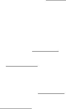
can be used instead. We have performed QCT calculations for obtaining integral cross-sections of the D þ H2 (v ¼ 1; jÞ ! DHðv0; j0Þ þ H reaction at the total energy of 1.8 eV (translational energy 1.0 eV) with the LSTH [75,76] potential energy parameters. These studies have been done with or without inclusion of the geometric phase and starting from initial states (v ¼ 1; j ¼ 1). For this case, 1:2 105 trajectories are taken noting that convergence was actually obtained with 5 104 trajectories. The distribution of integral cross-sections with (y0 ¼ 11:5 ) or without inclusion of the geometric phase as a function of j0 (v0 ¼ 1) has been shown in Figure 1 and compared with those QCT results obtained by using y0 ¼ 0.
In Figure 1, we see that there are relative shifts of the peak of the rotational distribution toward the left from j0 ¼ 12 to j0 ¼ 8 in the presence of the geometric phase. Thus, for the D þ H2 (v ¼ 1; j) ! DH ðv0; j0Þ þ H reaction with the same total energy 1.8 eV, we find qualitatively the same effect as found quantum mechanically. Kuppermann and Wu [46] showed that the peak of the
rotational state distribution moves toward the left in the presence of a geometric phase for the process D þ H2 (v ¼ 1; j ¼ 1Þ ! DH ðv0 ¼ 1; j0Þ þ H. It is important to note the effect of the position of the conical intersection (y0) on the
rotational distribution for the D þ H2 reaction. Although the absolute position of the peak (from j0 ¼ 10 to j0 ¼ 8) obtained from the quantum mechanical calculation is different from our results, it is worthwhile to see that the peak
Figure 1. Quasiclassical cross-sections for the reaction D þ H2 (v ¼ 1; j ¼ 1Þ ! DH ðv0 ¼ 1; j0Þ þ H at 1.8-eV total energy as a function of j0. The solid line indicates results obtained without including the geometric phase effect. Boxes show the results with the geometric phase included using either y0 ¼ 0 (dashed) or y0 ¼ 11:5 (dotted).