p365-detlefs(хижа)

The reader might hope that the first three lines of this procedure would be enough and that the rest of it is superfluous, but the following example shows otherwise:

In the tableau above, the unknown a is manifestly maximized at zero. When CloseRow is applied to a’s row, the first three lines kill the column owned by p. This leaves a nonminimal tableau, since the tableau then implies b = c = 0 and that q = −r. The rest of CloseRow will restore minimality by pivoting the tableau to make either b or c a column owner and killing the column.

As a historical note, the description in Nelson’s thesis [Nelson 1979] erroneously implied that CloseRow could be implemented with the first three lines alone. This bug was also present in our first implementation of Simplify and went unnoticed for a considerable time, but eventually an ESC example provoked the bug and we diagnosed and fixed it. We note here that the fix we implemented years ago is different from the implementation above, so the discrepancy between paper and code is greater in this section than in the rest of our description of the Simplex module.

As remarked above, AssertZ could be implemented with two calls to AssertGE. But if it were, the second of the two calls would always lead to a call to CloseRow, which would incur the cost of reminimizing the tableau by retesting the restricted unknowns. This work is not always necessary, as shown by the following lemma:

LEMMA 5. If an unknown u takes on both positive and negative values within TableauSoln, and a restricted unknown v is positive somewhere in TableauSoln, then (v > 0 u = 0) must hold somewhere in TableauSoln.

PROOF. Let P be a point in TableauSoln such that v(P) > 0. If u(P) = 0, we are done. Otherwise, let Q be a point in TableauSoln such that u(Q) has sign opposite to u(P). Since TableauSoln is convex, line segment PQ lies entirely within TableauSoln. Let R be the point on PQ such that u(R) = 0. Since v is restricted, v(Q) ≥ 0. Since v(Q) ≥ 0, v(P) > 0, R PQ, and R = Q, it follows that v(R) > 0.

We will provide an improved implementation of AssertZ that takes advantage of Lemma 5. The idea is to use two calls to SgnOfMax to determine the signs of the maximum and minimum of the argument. If these are positive and negative respectively, then by Lemma 5, we can perform the assertion by killing a single column. We will need to modify SgnOfMax to record in the globals (iLast, jLast) the row and column of the last pivot performed (if any). Since SgnOfMax(u) never performs any pivots after u acquires a positive sample value, and since pivoting is its own inverse, it follows that this modified SgnOfMax satisfies the additional postcondition:

If u’s initial sample value is at most zero, and u ends owning a row and 1 is returned, then the tableau is left in a state such that pivoting at (iLast, jLast) would preserve feasibility and make u’s sample value at most zero.

Using the modified SgnOfMax, we implement AssertZ as follows:

proc AssertZ(fas : formal affine sum of connected unknowns) ≡ var u := UnknownForFAS(fas) in

if u is manifestly equal to Zero then return

end;

var sgmx := SgnOfMax(u) in if sgmx < 0 then

refuted := true; return

else if sgmx = 0 then

CloseRow(u.index); return

else

//Sign of max of fas is positive. if u.ownsRow then

for j := 0 to m do

a[u.index, j] := −a[u.index, j] end;

else

for i := 1 to n do

a[i, u.index] := −a[i, u.index] end

end;

//u now represents −fas.

sgmx := SgnOfMax(u) in if sgmx < 0 then

refuted := true; return

else if sgmx = 0 then

CloseRow(u.index); return

else

// Sign of max of −fas is also positive, hence Lemma 5 applies. if u.ownsRow then

Pivot(u.index, jLast); end;

KillCol(u.index); return

end end

end end

end

The main advantage of this code for AssertZ over the two calls to AssertGE occurs in the case where both calls to SgnOfMax return 1. In this case, the unknown u takes on both positive and negative values over the initial TableauSoln, so we know by Lemma 5 that if any restricted unknown v is positive for some point in the initial TableauSoln, v is also positive at some point that remains in TableauSoln after the call to KillCol adds the dead column constraint u = 0. Thus, the minimality of the tableau is guaranteed to be preserved without any need for the loop over the restricted unknowns that would be caused by the second of the two AssertGE assertions.

We must also show that feasibility of the tableau is preserved in the case where both calls to SgnOfMax return 1. In this case, the first call to SgnOfMax leaves u

with sample value at least 0. After the entries in u’s row or column are negated, u then has sample value at most 0. If the second call to SgnOfMax then leaves u as a row owner, the postconditions of SgnOfMax guarantee that u ≥ 0 at the sample point, and that pivoting at (iLast, jLast) would move the sample point to a point on the line of variation (§8.3) of x[jLast] where u ≤ 0 while preserving feasibility. Instead, we pivot at (u.index, jLast), which moves the sample point to the point along the line of variation of x[jLast] to the point where u = 0. By the convexity of TableauSoln, this pivot also preserves feasibility.

A final fine point: The story we have told so far would require a tableau row for each distinct numeric constant appearing in the conjecture. In fact, Simplify incorporates an optimization that often avoids creating unknowns for numeric constants. A price of this optimization is that it becomes necessary to propagate equalities not only between unknowns but also between an unknown and a numeric constant. For example, when Simplify interns (§4.5) and asserts a literal containing the term f (6), it creates an E-node for the term 6 but does not connect it to a Simplex unknown. On the other hand, if the Simplex tableau later were to imply u = 6, for some connected unknown u, Simplify would then ensure that an equality is propagated between u.enode and the E-node for 6. The changes to CloseRow required to detect unknowns that have become “manifestly constant” are straightforward.

8.5. UNDOING TABLEAU OPERATIONS. The algorithms we have presented push undo records when they modify SignSoln, DColSoln, RowSoln, or the set of connected unknowns. In this section, we describe how these undo records are processed by Pop. Since the representation of Asserted is given as a function of SignSoln, DColSoln, RowSoln, it follows from the correctness of these bits of undoing code that Pop meets its specification of restoring Asserted.

Notice that we do not push an undo record for Pivot. As a consequence Pop may not restore the initial permutation of the row and column owners. This doesn’t matter as long as the semantics of SignSoln, DColSoln, RowSoln are restored.

To process an undo record of the form ("Unrestrict", u):

u.restricted := false.

To process an undo record of the form "ReviveCol":

dcol := dcol − 1.

To process an undo record of the form ("Deallocate", u):

if u.ownsRow then

copy row n to row u.index; y[u.index] := y[n];

n := n − 1

else if u’s column is identically 0 then copy column m to column u.index; x[u.index] := x[m];

m:= m − 1

else

perform some pivot in u’s column that preserves feasibility; copy row n to row u.index;

y[u.index] := y[n];

n:= n − 1

end;

if u.enode = nil then

u.enode.Simplex Unknown := nil; u.enode := nil

end

In arguing the correctness of this undo action, we observe that there are two cases in which an unknown is allocated: UnknownForEnode allocates a completely unconstrained unknown and connects it to an E-node, and UnknownForFAS allocates a constrained unknown and leaves it unconnected. If the unknown u to be deallocated was allocated by UnknownForEnode, then at entry to the action above the tableau will have been restored to a state where u is again completely unconstrained. In this case, u must own an identically zero column. All that is required to undo the forward action is to delete the vacuous column, which can be done by overwriting it with column m and decrementing m. If u was allocated by UnknownForFAS, then u will be constrained by RowSoln. If u happens to a row owner, we need only delete its row. If u owns a column, we cannot simply delete the column (since that would change the projection of RowSoln onto the remaining unknowns), so we must pivot u to make it a row owner. The argument that it is always possible to do this while preserving feasibility is similar to those for ToRow and for FindPivot, and we leave the details to the reader.

8.6. INTEGER HEURISTICS. As is well known, the satisfiability problem for linear inequalities over the rationals is solved in polynomial time by various ellipsoid methods and solved rapidly in practice by the Simplex method, but the same problem over the integers is NP-complete: Propositional unknowns can be constructed from integer unknowns by adding constraints like 0 ≤ b b ≤ 1, after which ¬ b is encoded 1 − b, and b c d is encoded b + c + d > 0. Thus, 3SAT is encoded.

For integer linear inequalities that arise from such an encoding, it seems extremely likely (as likely as P = NP) that the only way to solve the satisfiability problem will be by some kind of backtracking search. A fundamental assumption of Simplify is that most of the arithmetic satisfiability problems arising in program checking don’t resemble such encoded SAT problems and don’t require such a backtracking search.

In designing Simplify, we might have introduced a built-in monadic predicate characterizing the integers. Had we done so, a conjecture could mention both integer and rational unknowns. But rational unknowns did not seem useful in our program-checking applications. (We did not aspire to formulate a theory of floating-point numbers.) So Simplify treats all arithmetic arguments and results as integers.

The Simplex module’s satisfiability procedure is incomplete for integer linear arithmetic. However, by combining the complete decision procedure for rational linear arithmetic described above with three heuristics for integer arithmetic, we have obtained satisfactory results for our applications.

The first heuristic, the negated inequality heuristic, is that to assert a literal of the form ¬ a ≤ b, Simplify performs the call AssertGE(a − b − 1).

We found this heuristic alone to be satisfactory for a number of months. It is surprisingly powerful. For example, it allows proving the following formula:

i ≤ n f (i) = f (n) i ≤ n − 1.

The reason this formula is proved is that the only possible counterexample (§6.1)

i ≤ n, f (i) = f (n), ¬ i ≤ n − 1,

and the heuristically transformed third literal i − (n − 1) − 1 ≥ 0 combines with the first literal to propagate the equality i = n, contradicting the second literal.

Eventually, we encountered examples for which the negated inequality heuristic alone was insufficient. For example:

2 ≤ i f (i) = f (2) f (i) = f (3) 4 ≤ i.

We therefore added a second integer heuristic, the Tighten Bounds proof tactic. If, for some term t that is not an application of +, −, or ×, the Simplex tableau contains upper and lower bounds on t: L ≤ t and t ≤ U , for integer constants L and U , Simplify will try to refute the possibility t = L (not try so hard as to do a case split, but Simplify will do matching on both unit and nonunit matching rules (§5.2) in the attempted refutation), and if it is successful, it will then strengthen the lower bound from L to L + 1 and continue. It would be perfectly sound to apply the tactic to terms that were applications of +, −, or ×, but for efficiency’s sake we exclude them.

The Tighten Bounds tactic is given low priority. Initially, it had the lowest priority of all proof tactics: it was only tried as a last resort before printing a counterexample. However, we later encountered conjectures whose proof required the use of Tighten Bounds many times. We therefore introduced a Boolean recording whether the tactic had recently been useful. When this Boolean is true, the priority of the tactic is raised to just higher than case splitting. The Boolean is set to true whenever the Tighten Bounds tactic is successful, and it is reset to false when Simplify backtracks from a case split on a non-goal clause and the previous case split on the current path (§3.1) was on a goal (§3.5) clause. That is, the boolean is reset whenever clause scores are renormalized (as described in Section 3.6).

Simplify’s third integer arithmetic heuristic is the manifest constant heuristic. If all live column entries in some row of the tableau are zero, then the tableau implies that the row owner is equal to the entry in its constant column entry. If the constant column entry in such a row is not an integer, then the Simplex module detects a contradiction and sets refuted.

8.7. OVERF LOW. Simplify implements the rational numbers in the simplex tableau as ratios of 32-bit or 64-bit integers, depending on the platform. By default, Simplify does no overflow checking. If an overflow does occur it can produce a crash or an incorrect result. Several of the bug reports that we have received have been traced to such overflows. Simplify accepts a switch that causes it to check each tableau operation for overflow and halt with an error message if an overflow occurs. When ESC/Java is applied to its own front end, none of the proofs of the 2331 verification conditions overflows on a 64-bit machine; one of them overflows on a 32-bit machine. Enabling overflow checking increases total proof time by about four percent on the average.

9. Performance Measurements

In this section, we report on the performance of Simplify and on the performance effects of heuristics described in the rest of the article.

All performance figures in this section are from runs on a 500-MHz Compaq Alpha (EV6) with 5-GB main memory. The most memory used by Simplify on the “front-end test suite”, defined below, seems to be 100 MB. The machine has three processors, but Simplify is single-threaded. Simplify is coded in Modula-3 with all bounds checking and null-dereference checks enabled. Simplify relies on the Modula-3 garbage collector for storage management.

Our goal was to achieve performance sufficient to make the extended static checker useful. With the released version of Simplify, ESC/Java is able to check the 44794 thousand lines of Java source in its own front end (comprising 2331 routines and 29431 proof obligations) in 91 minutes. This is much faster than the code could be checked by a human design review, so we feel we have succeeded. We have no doubt that further performance improvements (even dramatic ones) are possible, but we stopped working on performance when Simplify became fast enough for ESC.

We used two test suites to produce the performance data in this section. The first suite, which we call the “small test suite” consists of five verification conditions (§1) generated by ESC/Modula-3 (addhi, cat, fastclose, frd-seek, simplex), eleven verification conditions generated by ESC-Java:

toString isCharType visitTryCatchStmt

binaryNumericPromotion Parse getRootInterface checkTypeDeclOfSig checkTypeDeclElem main

getNextPragma scanNumber

and two artificial tests (domino6x4x and domino6x6x) that reduce the well-known problem of tiling a mutilated checkerboard with 1-by-2 dominos into test cases that exercise case splitting and the E-graph. The second suite, which we call the “front-end test suite” consists of the 2331 verification conditions for the routines of ESC/Java’s front end. Both test suites contain valid conjectures only. These tests are available on the web [Detlefs et al. 2003a].

Much of our performance work aimed not so much at improving the average case as at steering clear of the worst case. Over the course of the ESC project, Simplify would occasionally “go off the deep end” by diving into a case analysis whose time to completion was wildly longer than any user would ever wait. When this happened, we would analyze the problem and the computation into which Simplify stumbled, and design a change that would prevent the problem from occurring. The change might not improve average case behavior, but we took the view that going off the deep end on extended static checking of realistic programs was worse than simple slowness.

Of course, it could be that the next realistic program that ESC is applied to will send Simplify off the deep end in a way that we never encountered and never took precautions against. Therefore, when ESC uses Simplify to check a routine, it sets a timeout. If Simplify exceeds the timeout, ESC notifies the user and goes on to

FIG. 4. Baseline performance data for the small test suite.

check the next routine. The default time limit used by ESC/Java, and in the tests reported in this section, is 300 seconds.

Many of the optimizations that Simplify employs can be disabled, and Simplify has other options and configurable parameters. In Sections 9.2 through 9.13, we evaluate the performance effects of the most important of these options. We don’t, of course, test every combination of options, but we have tried to test each option against the baseline behavior in which all options have their default values. Sections 9.14 through 9.17 discuss more general performance issues.

One of the verifications condition in the front end test suite requires approximately 400 seconds with Simplify’s default options, and thus times out with our 300-second time limit. No other test in either suite times out.

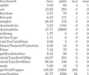
Figure 4 gives the baseline performance data for the tests in the small suite. For each benchmark, the figure presents the benchmark name, the time in seconds for Simplify to prove the benchmark, the number of case splits performed, the number of times during the proof that the matching depth (§5.2.1) was incremented, and the maximum matching depth that was reached.

9.1.SIMPLIFY AND OTHER PROVERS. As we go to press, Simplify is a rather old system. Several more recent systems that use decision procedures are substantially faster than Simplify on unquantified formulas. This was shown by a recent performance study performed by de Moura and Ruess [2004]. Even at its advanced age, Simplify seems to be a good choice for quantified formulas that require both matching and decision procedures.

9.2.PLUNGING. As described in Section 4.6, Simplify uses the plunging heuristic, which performs a Push-Assert-Pop sequence to test the consistency of a literal with the current context, in an attempt to refine the clause containing the literal. Plunging is more complete than the E-graph tests (§4.6), but also more expensive. By default Simplify plunges on each literal of each clause produced by matching a non-unit matching rule (§5.2): untenable literals are deleted from the clause, and if any literal’s negation is found untenable, the entire clause is deleted.

FIG. 5. Performance data for the small test suite with plunging disabled.

Early in Simplify’s history, we tried refining all clauses by plunging before doing each case-split. The performance of this strategy was so bad that we no longer even allow it to be enabled by a switch, and so cannot reproduce those results here.

We do have a switch that turns off plunging. Figure 5 compares, on the small test suite, the performance of Simplify with plunging disabled to the baseline. The figure has the same format as Figure 4 with an additional column that gives the percentage change in time from the baseline. The eighteen test cases of the small suite seem insufficient to support a firm conclusion. But, under the principle of steering clear of the worst case, the line for cat is a strong vote for plunging.

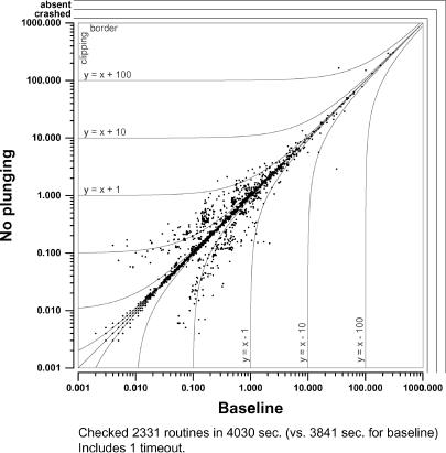
Figure 6 below illustrates the performance effect of plunging on each of the front end test suite. The figure contains one dot for each routine in the front end. The dot’s x-coordinate is the time required to prove that routine’s verification condition by the baseline Simplify and its y-coordinate is the time required by Simplify with plunging disabled. As the caption of the figure shows, plunging reduces the total time by about five percent. Moreover, in the upper right of the figure, all dots that are far from the diagonal are above the diagonal. Thus, plunging both improves the average case behavior and is favored by the principle of steering clear of the worst case.

The decision to do refinement by plunging still leaves open the question of how much effort should be expended during plunging in looking for a contradiction. If asserting the literal leads to a contradiction in one of Simplify’s built-in theory modules, then the matter is settled. But if not, how many inference steps will be attempted before admitting that the literal seems consistent with the context? Simplify has several options, controlled by a switch. Each option calls AssertLit, then performs some set of tactics to quiescence, or until a contradiction is detected. Here’s the list of options (each option includes all the tactics the preceding option).

0Perform domain-specific decision procedures and propagate equalities.

1Call (a nonplunging version of) Refine.

2Match on unit rules (§5.2).

3Match on non-unit rules (but do not plunge on their instances).

FIG. 6. Effect of disabling plunging on the front-end test suite.

Simplify’s default is option 0, which is also the fastest of the options on the frontend test suite. However, option 0, option 1, and no plunging at all are all fairly close. Option 2 is about twenty percent worse, and option 3 is much worse, leading to many timeouts on the front-end test suite.

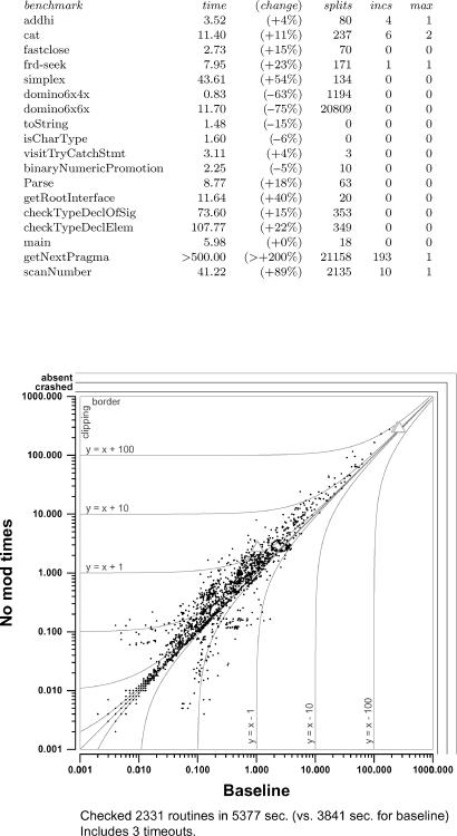
9.3. THE MOD-TIME OPTIMIZATION. As described in Section 5.4.2, Simplify use the mod-time optimization, which records modification times in E-nodes in order to avoid fruitlessly searching for new matches in unchanged portions of the E-graph. Figure 7 shows the elapsed times with and without the mod-time optimization for Simplify on our small test suite.

For the two domino problems, there is no matching, and therefore the mod-time feature is all cost and no benefit. It is therefore no surprise that mod-time updating caused a slowdown on these examples. The magnitude of the slowdown is, at least to us, a bit of a surprise, and suggests that the mod-time updating code is not as tight as it could be. Despite this, on all the cases derived from program checking, the mod-time optimization was either an improvement (sometimes quite significant) or an insignificant slowdown.

Figure 8 shows the effect of disabling the mod-time optimization on the front-end test suite. Grey triangles are used instead of dots if the outcome of the verification is different in the two runs. In Figure 8, the two triangles in the upper right corner are cases where disabling the mod-time optimization caused timeouts. The hard-to-see