

|
|
|
|
C H A P T E R 1 |
The Science of Macroeconomics | 7 |
|||||
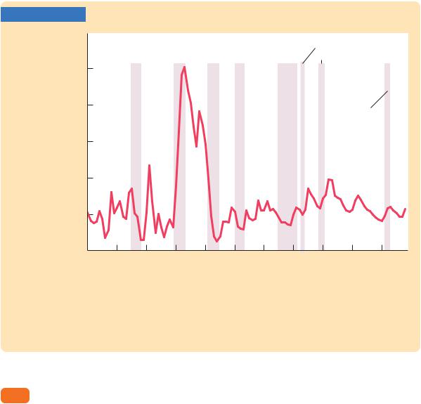
FIGURE 1-3 |
|
|
|
|
|
|
|
|
|
|
Percent unemployed |
|
World |
Great |
World |
Korean |
|
Vietnam |
First oil price shock |
||
|
|
|
||||||||
|
|
War I |
Depression |
War II |
War |
|
War |
Second oil price shock |
||
25 |
|
|
|
|
|
|
|
|
|
|
20 |
|
|
|
|
|
|
|
|
9/11 |
|
|
|
|
|
|
|
|
|
|
|
|
|
|
|
|
|
|
|
|
|
terrorist |
|
|
|
|
|
|
|
|
|
|
attack |
|
15 |
|
|
|
|
|
|
|
|
|
|
10 |
|
|
|
|
|
|
|
|
|
|
5 |
|
|
|
|
|
|
|
|
|
|
0 |
1910 |
1920 |
1930 |
1940 |
1950 |
1960 |
1970 |
1980 |
1990 |
2000 |
1900 |
||||||||||
|
|
|
|
|
|
|
|
|
|
Year |
The Unemployment Rate in the U.S. Economy The unemployment rate measures the percentage of people in the labor force who do not have jobs. This figure shows that the economy always has some unemployment and that the amount fluctuates from year to year.
Source: U.S. Department of Labor and U.S. Bureau of the Census (Historical Statistics of the United States: Colonial Times to 1970).
1-2 How Economists Think
Economists often study politically charged issues, but they try to address these issues with a scientist’s objectivity. Like any science, economics has its own set of tools—terminology, data, and a way of thinking—that can seem foreign and arcane to the layman.The best way to become familiar with these tools is to practice using them, and this book affords you ample opportunity to do so.To make these tools less forbidding, however, let’s discuss a few of them here.
Theory as Model Building
Young children learn much about the world around them by playing with toy versions of real objects. For instance, they often put together models of cars, trains, or planes. These models are far from realistic, but the model-builder
8 | P A R T I Introduction
learns a lot from them nonetheless.The model illustrates the essence of the real object it is designed to resemble. (In addition, for many children, building models is fun.)
Economists also use models to understand the world, but an economist’s model is more likely to be made of symbols and equations than plastic and glue. Economists build their “toy economies” to help explain economic variables, such as GDP, inflation, and unemployment. Economic models illustrate, often in mathematical terms, the relationships among the variables. Models are useful because they help us to dispense with irrelevant details and to focus on underlying connections. (In addition, for many economists, building models is fun.)
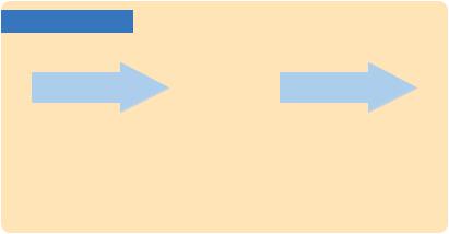
Models have two kinds of variables: endogenous variables and exogenous variables. Endogenous variables are those variables that a model tries to explain. Exogenous variables are those variables that a model takes as given. The purpose of a model is to show how the exogenous variables affect the endogenous variables. In other words, as Figure 1-4 illustrates, exogenous variables come from outside the model and serve as the model’s input, whereas endogenous variables are determined within the model and are the model’s output.
FIGURE 1-4
|
|
|
Exogenous Variables |
Model |
Endogenous Variables |
|
|
|
|
|
|
How Models Work Models are simplified theories that show the key relationships among economic variables. The exogenous variables are those that come from outside the model. The endogenous variables are those that the model explains. The model shows how changes in the exogenous variables affect the endogenous variables.
To make these ideas more concrete, let’s review the most celebrated of all economic models—the model of supply and demand. Imagine that an economist wanted to figure out what factors influence the price of pizza and the quantity of pizza sold. He or she would develop a model that described the behavior of pizza buyers, the behavior of pizza sellers, and their interaction in the market for pizza. For example, the economist supposes that the quantity of pizza demanded by consumers Qd depends on the price of pizza P and on aggregate income Y. This relationship is expressed in the equation
Qd = D(P, Y ),
where D( ) represents the demand function. Similarly, the economist supposes that the quantity of pizza supplied by pizzerias Qs depends on the price of pizza P
C H A P T E R 1 The Science of Macroeconomics | 9
and on the price of materials Pm, such as cheese, tomatoes, flour, and anchovies. This relationship is expressed as
Qs = S(P, Pm),
where S( ) represents the supply function. Finally, the economist assumes that the price of pizza adjusts to bring the quantity supplied and quantity demanded into balance:
Qs = Qd.
These three equations compose a model of the market for pizza.
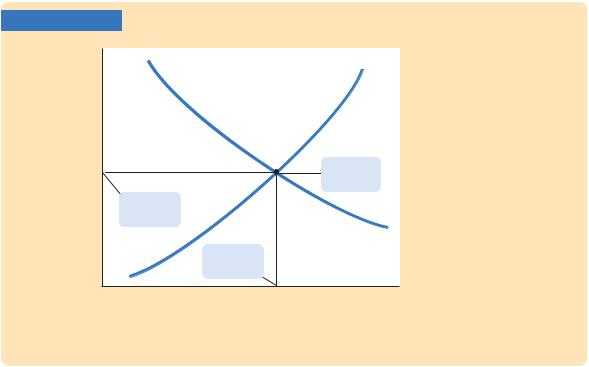
The economist illustrates the model with a supply-and-demand diagram, as in Figure 1-5. The demand curve shows the relationship between the quantity of pizza demanded and the price of pizza, holding aggregate income constant. The demand curve slopes downward because a higher price of pizza encourages consumers to switch to other foods and buy less pizza. The supply curve shows the relationship between the quantity of pizza supplied and the price of pizza, holding the price of materials constant. The supply curve slopes upward because a higher price of pizza makes selling pizza more profitable, which encourages pizzerias to produce more of it. The equilibrium for the market is the price and quantity at which the supply and demand curves intersect. At the equilibrium price, consumers choose to buy the amount of pizza that pizzerias choose to produce.
This model of the pizza market has two exogenous variables and two endogenous variables. The exogenous variables are aggregate income and the price of
FIGURE 1-5
Price of pizza, P
Supply
Market equilibrium
Equilibrium price
Demand
Equilibrium quantity
Quantity of pizza, Q
The Model of Supply and Demand The most famous economic model is that of supply and demand for a good or service—in this case, pizza. The demand curve is a downward-sloping curve relating the price of pizza to the quantity of pizza that consumers demand. The supply curve is an upward-sloping curve relating the price of pizza to the quantity of pizza that pizzerias supply. The price of pizza adjusts until the quantity supplied equals the quantity demanded. The point where the two curves cross is the market equilibrium, which shows the equilibrium price of pizza and the equilibrium quantity of pizza.
10 | P A R T I Introduction
materials.The model does not attempt to explain them but instead takes them as given (perhaps to be explained by another model).The endogenous variables are the price of pizza and the quantity of pizza exchanged. These are the variables that the model attempts to explain.
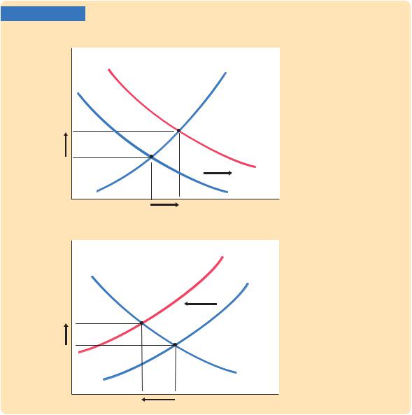
The model can be used to show how a change in one of the exogenous variables affects both endogenous variables. For example, if aggregate income increases, then the demand for pizza increases, as in panel (a) of Figure 1-6.The model shows that both the equilibrium price and the equilibrium quantity of pizza rise. Similarly, if the price of materials increases, then the supply of pizza decreases, as in panel (b) of Figure 1-6. The model shows that in this case the
FIGURE 1-6
Price of pizza, P
P2
P1
Price of pizza, P
P2
P1
(a) A Shift in Demand
S
D2
D1
Q1 |
Q2 |
Quantity of pizza, Q |
(b) A Shift in Supply
S2
S1
|
|
D |
Q2 |
Q1 |
Quantity of pizza, Q |
Changes in Equilibrium In panel (a), a rise in aggregate income causes the demand for pizza to increase: at any given price, consumers now want to buy more pizza. This is represented by a rightward shift in the demand curve from D1 to D2. The market moves to the new intersection of supply and demand. The equilibrium price rises from P1 to P2, and the equilibrium quantity of pizza rises from Q1 to Q2. In panel (b), a rise in the price of materials decreases the supply of pizza: at any given price, pizzerias find that the sale of pizza is less profitable and therefore choose to produce less pizza. This is represented by a leftward shift in the supply curve from S1 to S2. The market moves to the new intersection of supply and demand. The equilibrium price rises from P1 to P2, and the equilibrium quantity falls from Q1 to Q2.

C H A P T E R 1 The Science of Macroeconomics | 11
equilibrium price of pizza rises and the equilibrium quantity of pizza falls.Thus, the model shows how changes either in aggregate income or in the price of materials affect price and quantity in the market for pizza.
Like all models, this model of the pizza market makes simplifying assumptions. The model does not take into account, for example, that every pizzeria is in a different location. For each customer, one pizzeria is more convenient than the others, and thus pizzerias have some ability to set their own prices. The model assumes that there is a single price for pizza, but in fact there could be a different price at every pizzeria.
How should we react to the model’s lack of realism? Should we discard the simple model of pizza supply and demand? Should we attempt to build a more complex model that allows for diverse pizza prices? The answers to these questions depend on our purpose. If our goal is to explain how the price of cheese affects the average price of pizza and the amount of pizza sold, then the diversity of pizza prices is probably not important.The simple model of the pizza market does a good job of addressing that issue. Yet if our goal is to explain why towns with ten pizzerias have lower pizza prices than towns with two, the simple model is less useful.
FYI
Using Functions to Express Relationships Among Variables
All economic models express relationships among economic variables. Often, these relationships are expressed as functions. A function is a mathematical concept that shows how one variable depends on a set of other variables. For example, in the model of the pizza market, we said that the quantity of pizza demanded depends on the price of pizza and on aggregate income. To express this, we use functional notation to write
Qd = D(P, Y).
This equation says that the quantity of pizza demanded Qd is a function of the price of pizza P and aggregate income Y. In functional notation, the variable preceding the parentheses denotes the function. In this case, D( ) is the function expressing how the variables in parentheses determine the quantity of pizza demanded.
If we knew more about the pizza market, we could give a numerical formula for the quantity of pizza demanded. For example, we might be able to write
Qd = 60 − 10P + 2Y.
In this case, the demand function is
D(P, Y ) = 60 − 10P + 2Y.
For any price of pizza and aggregate income, this function gives the corresponding quantity of pizza demanded. For example, if aggregate income is $10 and the price of pizza is $2, then the quantity of pizza demanded is 60 pies; if the price of pizza rises to $3, the quantity of pizza demanded falls to 50 pies.
Functional notation allows us to express the general idea that variables are related, even when we do not have enough information to indicate the precise numerical relationship. For example, we might know that the quantity of pizza demanded falls when the price rises from $2 to $3, but we might not know by how much it falls. In this case, functional notation is useful: as long as we know that a relationship among the variables exists, we can express that relationship using functional notation.