

43.Perfect competition
Firms in perfect competition face the maximum amount of competition because there are many competing firms, each of which produces an identical product.
Firms in perfect competition maximize their profit by producing where MR = MC.
Perfect competition leads to an efficient allocation of resources.
I. What is Perfect Competition?
Perfect competition is an industry in which
Many firms sell identical products to many buyers
There are no restrictions on entry into the industry
Established firms have no advantage over existing ones
Sellers and buyers are well informed about prices
These characteristics of perfect competition arise when the minimum efficient scale for a firm is small relative to the size of the entire market.
Firms operating in perfect competition seek to maximize economic profit, which is the difference between total revenue (the price of the firm’s output multiplied by the quantity sold) and its total opportunity cost of production.
Firms in perfect competition are price takers, meaning that a firm that cannot influence the market price and so it sets its own price equal to the market price.
Because the firm is a price taker, its marginal revenue—which is the change in total revenue that results in a one-unit increase in the quantity sold—is equal to the market price and remains constant as output sold increases. The firm’s demand is perfectly elastic and the firm’s demand curve is a horizontal line at the market price.
44.The firm’s output decision
Marginal Analysis and the Supply Decision
The firm produces the quantity of output for which the difference between total revenue and total cost is at its maximum because this difference is its economic profit.
Marginal analysis can be used to determine the profit maximizing quantity. The firm compares the marginal revenue (which remains constant with output) to the marginal cost (which changes with output) of producing different levels of output.
When MR > MC, then the extra revenue from selling one more unit exceeds the extra cost of producing one more unit, so the firm increases its output to increase its profit.
When MR < MC, then the extra cost of producing one more unit exceeds the extra revenue from selling one more unit, so the firm decreases its output to increase its profits
When MR = MC, then the extra cost of producing one more unit equals the extra revenue from selling one more unit, so the firm’s profit is maximized at this level of output.
I
 n
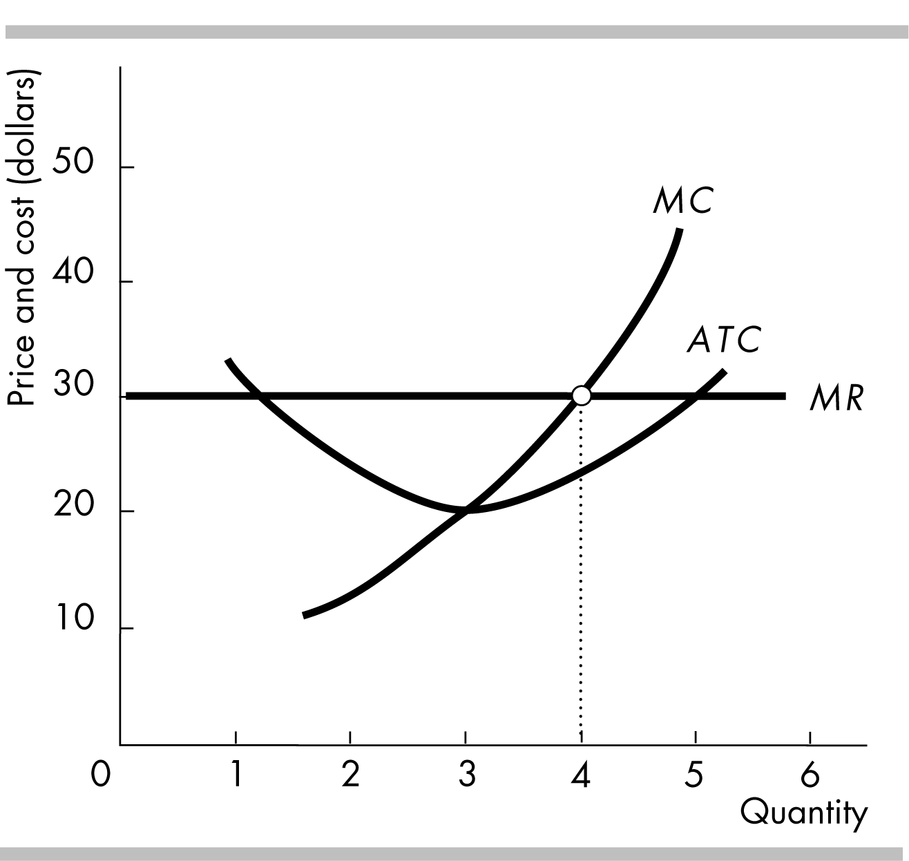
the figure the firm produces 4 units of output because that is the
quantity that sets the firm’s marginal cost equal to its marginal
revenue, that is, MR
= MC.
The firm then charges the going market price of $30 for its
product.
n
the figure the firm produces 4 units of output because that is the
quantity that sets the firm’s marginal cost equal to its marginal
revenue, that is, MR
= MC.
The firm then charges the going market price of $30 for its
product.
Temporary Shutdown Decision
The firm will temporarily shut down in the short run when price falls below the shutdown point, which is the output and price that just allows the firm to cover its total variable cost. The minimum AVC is the lowest price at which the firm will operate because if it operated with a lower price, the firm’s loss would be greater than if it shut down. (The loss when the firm shuts down is equal to its fixed cost.)
The firm will continue operating in the short run even if it incurs an economic loss as long as the price exceeds the minimum AVC.
The Firm’s Supply Curve
As long as the firm remains open, it produces where MR = MC. So the firm’s supply curve is its MC curve above the minimum AVC. At prices below the minimum AVC, the firm shuts down and supplies zero.
The figure shows the firm’s supply curve as the heavy dark line.
At prices less than the minimum average variable cost, which equals P in the figure, the firm shuts down and supplies zero.
At prices greater than the minimum average variable cost, the firm supplies along its marginal cost curve. Hence the firm’s marginal cost curve is its supply, indicated in the figure by the S = MC curve.

The short-run market supply curve shows the quantity supplied by all the firms in the market at each price when each firm’s plant and number of firms remain the same. The quantity supplied in the industry at any price is the summation of all quantities supplied by each firm at that price, so the short-run industry supply curve is the horizontal summation of all the firms’ supply curves.
Changes in market demand influence the output and the entry or exit decisions made by firms. An increase in market demand shifts the demand curve rightward and raises the market price. Each firm in the industry responds by increasing its quantity supplied.
The higher price now exceeds each firm’s minimum ATC and the firms in the industry earn an economic profit. The figure illustrates a perfectly competitive firm earning an economic profit. The firm’s economic profit is equal to the area of the darkened rectangle.
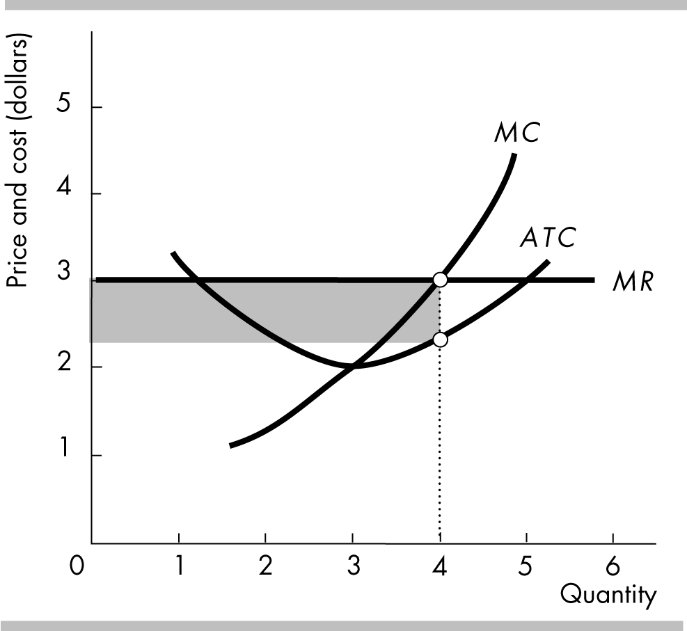
In the short run there are three possible profit outcomes—an economic profit, zero economic profit, and an economic loss.
If the price exceeds the ATC, the firm earns an economic profit (as illustrated in the figure).
If the price equals the ATC, the firm “breaks even” by earning zero economic profit. In this case, the firm earns a normal profit. At the profit maximizing level of output, q, the price, P, equals the ATC.
If the price is less than the ATC, the firm incurs an economic loss.