

euclid.ss.1009213726
.pdfSTATISTICAL MODELING: THE TWO CULTURES |
209 |
class #2 are x 2 . If these two sets of vectors can be separated by a hyperplane then there is an optimal separating hyperplane. “Optimal” is defined as meaning that the distance of the hyperplane to any prediction vector is maximal (see below).
The set of vectors in x 1 and in x 2 that achieve the minimum distance to the optimal separating hyperplane are called the support vectors. Their coordinates determine the equation of the hyperplane. Vapnik (1995) showed that if a separating hyperplane exists, then the optimal separating hyperplane has low generalization error (see Glossary).
optimal hyperplane
support vector
In two-class data, separability by a hyperplane does not often occur. However, let us increase the dimensionality by adding as additional predictor variables all quadratic monomials in the original predictor variables; that is, all terms of the form xm1xm2. A hyperplane in the original variables plus quadratic monomials in the original variables is a more complex creature. The possibility of separation is greater. If no separation occurs, add cubic monomials as input features. If there are originally 30 predictor variables, then there are about 40,000 features if monomials up to the fourth degree are added.
The higher the dimensionality of the set of features, the more likely it is that separation occurs. In the ZIP Code data set, separation occurs with fourth degree monomials added. The test set error is 4.1%. Using a large subset of the NIST data base as a training set, separation also occurred after adding up to fourth degree monomials and gave a test set error rate of 1.1%.
Separation can always be had by raising the dimensionality high enough. But if the separating hyperplane becomes too complex, the generalization error becomes large. An elegant theorem (Vapnik, 1995) gives this bound for the expected generalization error:
Ex GE ≤ Ex number of support vectors / N − 1
where N is the sample size and the expectation is over all training sets of size N drawn from the same underlying distribution as the original training set.
The number of support vectors increases with the dimensionality of the feature space. If this number
becomes too large, the separating hyperplane will not give low generalization error. If separation cannot be realized with a relatively small number of support vectors, there is another version of support vector machines that defines optimality by adding a penalty term for the vectors on the wrong side of the hyperplane.
Some ingenious algorithms make finding the optimal separating hyperplane computationally feasible. These devices reduce the search to a solution of a quadratic programming problem with linear inequality constraints that are of the order of the number N of cases, independent of the dimension of the feature space. Methods tailored to this particular problem produce speed-ups of an order of magnitude over standard methods for solving quadratic programming problems.
Support vector machines can also be used to provide accurate predictions in other areas (e.g., regression). It is an exciting idea that gives excellent performance and is beginning to supplant the use of neural nets. A readable introduction is in Cristianini and Shawe-Taylor (2000).
11. INFORMATION FROM A BLACK BOX
The dilemma posed in the last section is that the models that best emulate nature in terms of predictive accuracy are also the most complex and inscrutable. But this dilemma can be resolved by realizing the wrong question is being asked. Nature forms the outputs y from the inputs x by means of a black box with complex and unknown interior.
y |
|
nature |
|
|
x |
|
|
|
|||
|
|
|
|
|
|
Current accurate prediction methods are also complex black boxes.
neural nets
y forests
  x support vectors
So we are facing two black boxes, where ours seems only slightly less inscrutable than nature’s. In data generated by medical experiments, ensembles of predictors can give cross-validated error rates significantly lower than logistic regression. My biostatistician friends tell me, “Doctors can interpret logistic regression.” There is no way they can interpret a black box containing fifty trees hooked together. In a choice between accuracy and interpretability, they’ll go for interpretability.
Framing the question as the choice between accuracy and interpretability is an incorrect interpretation of what the goal of a statistical analysis is.
210 |
L. BREIMAN |
The point of a model is to get useful information about the relation between the response and predictor variables. Interpretability is a way of getting information. But a model does not have to be simple to provide reliable information about the relation between predictor and response variables; neither does it have to be a data model.
• The goal is not interpretability, but accurate information.
The following three examples illustrate this point. The first shows that random forests applied to a medical data set can give more reliable information about covariate strengths than logistic regression. The second shows that it can give interesting information that could not be revealed by a logistic regression. The third is an application to a microarray data where it is difficult to conceive of a data model that would uncover similar information.
11.1Example I: Variable Importance in a Survival Data Set
The data set contains survival or nonsurvival of 155 hepatitis patients with 19 covariates. It is available at ftp.ics.uci.edu/pub/MachineLearningDatabases and was contributed by Gail Gong. The description is in a file called hepatitis.names. The data set has been previously analyzed by Diaconis and Efron (1983), and Cestnik, Konenenko and Bratko (1987). The lowest reported error rate to date, 17%, is in the latter paper.
Diaconis and Efron refer to work by Peter Gregory of the Stanford Medical School who analyzed this data and concluded that the important variables were numbers 6, 12, 14, 19 and reports an estimated 20% predictive accuracy. The variables were reduced in two stages—the first was by informal data analysis. The second refers to a more formal
(unspecified) statistical procedure which I assume was logistic regression.
Efron and Diaconis drew 500 bootstrap samples from the original data set and used a similar procedure to isolate the important variables in each bootstrapped data set. The authors comment, “Of the four variables originally selected not one was selected in more than 60 percent of the samples. Hence the variables identified in the original analysis cannot be taken too seriously.” We will come back to this conclusion later.
Logistic Regression
The predictive error rate for logistic regression on the hepatitis data set is 17.4%. This was evaluated by doing 100 runs, each time leaving out a randomly selected 10% of the data as a test set, and then averaging over the test set errors.
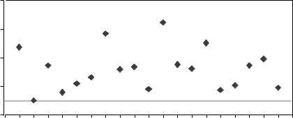
Usually, the initial evaluation of which variables are important is based on examining the absolute values of the coefficients of the variables in the logistic regression divided by their standard deviations. Figure 1 is a plot of these values.
The conclusion from looking at the standardized coefficients is that variables 7 and 11 are the most important covariates. When logistic regression is run using only these two variables, the cross-validated error rate rises to 22.9%. Another way to find important variables is to run a best subsets search which, for any value k, finds the subset of k variables having lowest deviance.
This procedure raises the problems of instability and multiplicity of models (see Section 7.1). There are about 4,000 subsets containing four variables. Of these, there are almost certainly a substantial number that have deviance close to the minimum and give different pictures of what the underlying mechanism is.
standardized coefficients
3.5
2.5
1.5
. 5
– . 5 |
|
|
|
|
|
|
|
|
|
|
|
|
|
|
|
|
|
|
|
|
0 |
1 |
2 |
3 |
4 |
5 |
6 |
7 |
8 |
9 |
1 0 |
1 1 |
1 2 |
1 3 |
1 4 |
1 5 |
1 6 |
1 7 |
1 8 |
1 9 |
2 0 |
variables
Fig. 1. Standardized coefficients logistic regression.
percent increse in error
STATISTICAL MODELING: THE TWO CULTURES |
211 |
5 0
4 0
3 0
2 0
1 0
0
– 1 0
0 |
1 |
2 |
3 |
4 |
5 |
6 |
7 |
8 |
9 |
1 0 |
1 1 |
1 2 |
1 3 |
1 4 |
1 5 |
1 6 |
1 7 |
1 8 |
1 9 |
2 0 |
variables
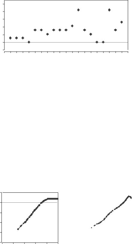
Fig. 2. Variable importance-random forest.
Random Forests
The random forests predictive error rate, evaluated by averaging errors over 100 runs, each time leaving out 10% of the data as a test set, is 12.3%— almost a 30% reduction from the logistic regression error.
Random forests consists of a large number of randomly constructed trees, each voting for a class. Similar to bagging (Breiman, 1996), a bootstrap sample of the training set is used to construct each tree. A random selection of the input variables is searched to find the best split for each node.
To measure the importance of the mth variable, the values of the mth variable are randomly permuted in all of the cases left out in the current bootstrap sample. Then these cases are run down the current tree and their classification noted. At the end of a run consisting of growing many trees, the percent increase in misclassification rate due to noising up each variable is computed. This is the
|
|
VARIABLE 12 vs PROBABILITY #1 |
|
|||
|
1 |
|
|
|
|
|
|
0 |
|
|
|
|
|
12 |
– 1 |
|
|
|
|
|
variable |
|
|
|
|
|
|
– 2 |
|
|
|
|
|
|
|
|
|
|
|
|
|
|
– 3 |
|
|
|
|
|
|
– 4 |
|
|
|
|
|
|
0 |
. 2 |
. 4 |
. 6 |
. 8 |
1 |
|
|
class 1 probability |
|
|
||
measure of variable importance that is shown in Figure 1.
Random forests singles out two variables, the 12th and the 17th, as being important. As a verification both variables were run in random forests, individually and together. The test set error rates over 100 replications were 14.3% each. Running both together did no better. We conclude that virtually all of the predictive capability is provided by a single variable, either 12 or 17.
To explore the interaction between 12 and 17 a bit further, at the end of a random forest run using all variables, the output includes the estimated value of the probability of each class vs. the case number. This information is used to get plots of the variable values (normalized to mean zero and standard deviation one) vs. the probability of death. The variable values are smoothed using a weighted linear regression smoother. The results are in Figure 3 for variables 12 and 17.
VARIABLE 17 vs PROBABILITY #1
|
1 |
|
|
|
|
|
|
|
|
|
|
|
|
|
|
|
|
|
|
|
|
|
|
|
|
|
|
|
|
|
|
|
|
|
|
|
|
|
|
|
|
17 |
0 |
|
|
|
|
|
|
|
|
|
|
|
|
|
|
|
|
|
|
|
|
|
|
|
|
|
|
|
|
|
|
|
|
|
|
|
|
|
|
||
|
|
|
|
|
|
|
|
|
|
|
|
|
|
|
|
|
|
|
||
|
|
|
|
|
|
|
|
|
|
|
|
|
|
|
|
|
|
|
|
|
variable |
– 1 |
|
|
|
|
|
|
|
|
|
|
|
|
|
|
|
|
|
|
|
|
|
|
|
|
|
|
|
|
|
|
|
|
|
|
|
|
|
|
||
|
|
|
|
|
|
|
|
|
|
|
|
|
|
|
|
|
|
|
|
|
|
– 2 |
|
|
|
|
|
|
|
|
|
|
|
|
|
|
|
|
|
|
|
|
|
|
|
|
|
|
|
|
|
|
|
|
|
|
|
|
|
|
|
|
|
– 3 |
|
|
|
|
|
|
|
|
|
|
|
|
|
|
|
|
|
|
|
|
|
|
|
|
|
|
|
|
|
|
|
|
|
|
|
|
|
|
|
|
|
0 |
. 2 |
. 4 |
. 6 |
. 8 |
1 |
||||||||||||||
|
|
|
|
|
|
|
|
class 1 probability |
|
|
|
|
|
|
||||||
Fig. 3. Variable 17 vs. probability #1.
212 |
L. BREIMAN |
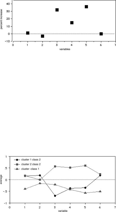
Fig. 4. Variable importance—Bupa data.
The graphs of the variable values vs. class death probability are almost linear and similar. The two variables turn out to be highly correlated. Thinking that this might have affected the logistic regression results, it was run again with one or the other of these two variables deleted. There was little change.
Out of curiosity, I evaluated variable importance in logistic regression in the same way that I did in random forests, by permuting variable values in the 10% test set and computing how much that increased the test set error. Not much help— variables 12 and 17 were not among the 3 variables ranked as most important. In partial verification of the importance of 12 and 17, I tried them separately as single variables in logistic regression. Variable 12 gave a 15.7% error rate, variable 17 came in at 19.3%.
To go back to the original Diaconis–Efron analysis, the problem is clear. Variables 12 and 17 are surrogates for each other. If one of them appears important in a model built on a bootstrap sample, the other does not. So each one’s frequency of occurrence
is automatically less than 50%. The paper lists the variables selected in ten of the samples. Either 12 or 17 appear in seven of the ten.
11.2 Example II Clustering in Medical Data
The Bupa liver data set is a two-class biomedical data set also available at ftp.ics.uci.edu/pub/MachineLearningDatabases. The covariates are:
1. |
mcv |
mean corpuscular volume |
2. |
alkphos |
alkaline phosphotase |
3. |
sgpt |
alamine aminotransferase |
4. |
sgot |
aspartate aminotransferase |
5. |
gammagt |
gamma-glutamyl transpeptidase |
6. |
drinks |
half-pint equivalents of alcoholic |
|
|
beverage drunk per day |
The first five attributes are the results of blood tests thought to be related to liver functioning. The 345 patients are classified into two classes by the severity of their liver malfunctioning. Class two is severe malfunctioning. In a random forests run,
Fig. 5. Cluster averages—Bupa data.
STATISTICAL MODELING: THE TWO CULTURES |
213 |
the misclassification error rate is 28%. The variable importance given by random forests is in Figure 4.
Blood tests 3 and 5 are the most important, followed by test 4. Random forests also outputs an intrinsic similarity measure which can be used to cluster. When this was applied, two clusters were discovered in class two. The average of each variable is computed and plotted in each of these clusters in Figure 5.
An interesting facet emerges. The class two subjects consist of two distinct groups: those that have high scores on blood tests 3, 4, and 5 and those that have low scores on those tests.
11.3 Example III: Microarray Data
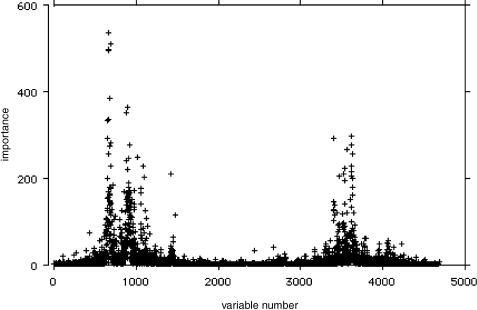
Random forests was run on a microarray lymphoma data set with three classes, sample size of 81 and 4,682 variables (genes) without any variable selection [for more information about this data set, see Dudoit, Fridlyand and Speed, (2000)]. The error rate was low. What was also interesting from a scientific viewpoint was an estimate of the importance of each of the 4,682 gene expressions.
The graph in Figure 6 was produced by a run of random forests. This result is consistent with assessments of variable importance made using other algorithmic methods, but appears to have sharper detail.
11.4 Remarks about the Examples
The examples show that much information is available from an algorithmic model. Friedman
(1999) derives similar variable information from a different way of constructing a forest. The similarity is that they are both built as ways to give low predictive error.
There are 32 deaths and 123 survivors in the hepatitis data set. Calling everyone a survivor gives a baseline error rate of 20.6%. Logistic regression lowers this to 17.4%. It is not extracting much useful information from the data, which may explain its inability to find the important variables. Its weakness might have been unknown and the variable importances accepted at face value if its predictive accuracy was not evaluated.
Random forests is also capable of discovering important aspects of the data that standard data models cannot uncover. The potentially interesting clustering of class two patients in Example II is an illustration. The standard procedure when fitting data models such as logistic regression is to delete variables; to quote from Diaconis and Efron (1983) again, “ statistical experience suggests that it is unwise to fit a model that depends on 19 variables with only 155 data points available.” Newer methods in machine learning thrive on variables—the more the better. For instance, random forests does not overfit. It gives excellent accuracy on the lymphoma data set of Example III which has over 4,600 variables, with no variable deletion and is capable of extracting variable importance information from the data.
Fig. 6. Microarray variable importance.
214 |
L. BREIMAN |
These examples illustrate the following points:
•Higher predictive accuracy is associated with more reliable information about the underlying data mechanism. Weak predictive accuracy can lead to questionable conclusions.
•Algorithmic models can give better predictive accuracy than data models, and provide better information about the underlying mechanism.
12. FINAL REMARKS
The goals in statistics are to use data to predict and to get information about the underlying data mechanism. Nowhere is it written on a stone tablet what kind of model should be used to solve problems involving data. To make my position clear, I am not against data models per se. In some situations they are the most appropriate way to solve the problem. But the emphasis needs to be on the problem and on the data.
Unfortunately, our field has a vested interest in data models, come hell or high water. For instance, see Dempster’s (1998) paper on modeling. His position on the 1990 Census adjustment controversy is particularly interesting. He admits that he doesn’t know much about the data or the details, but argues that the problem can be solved by a strong dose of modeling. That more modeling can make errorridden data accurate seems highly unlikely to me.
Terrabytes of data are pouring into computers from many sources, both scientific, and commercial, and there is a need to analyze and understand the data. For instance, data is being generated at an awesome rate by telescopes and radio telescopes scanning the skies. Images containing millions of stellar objects are stored on tape or disk. Astronomers need automated ways to scan their data to find certain types of stellar objects or novel objects. This is a fascinating enterprise, and I doubt if data models are applicable. Yet I would enter this in my ledger as a statistical problem.
The analysis of genetic data is one of the most challenging and interesting statistical problems around. Microarray data, like that analyzed in Section 11.3 can lead to significant advances in understanding genetic effects. But the analysis of variable importance in Section 11.3 would be difficult to do accurately using a stochastic data model.
Problems such as stellar recognition or analysis of gene expression data could be high adventure for statisticians. But it requires that they focus on solving the problem instead of asking what data model they can create. The best solution could be an algorithmic model, or maybe a data model, or maybe a
combination. But the trick to being a scientist is to be open to using a wide variety of tools.
The roots of statistics, as in science, lie in working with data and checking theory against data. I hope in this century our field will return to its roots. There are signs that this hope is not illusory. Over the last ten years, there has been a noticeable move toward statistical work on real world problems and reaching out by statisticians toward collaborative work with other disciplines. I believe this trend will continue and, in fact, has to continue if we are to survive as an energetic and creative field.
GLOSSARY
Since some of the terms used in this paper may not be familiar to all statisticians, I append some definitions.
Infinite test set error. Assume a loss function L y yˆ that is a measure of the error when y is the true response and yˆ the predicted response. In classification, the usual loss is 1 if y = yˆ and zero if y = yˆ. In regression, the usual loss isy − yˆ2. Given a set of data (training set) consisting of yn xn n = 1 2 N , use it to construct a predictor function φ x of y. Assume that the training set is i.i.d drawn from the distribution of the random vector Y X. The infinite test set error is E L Y φ X . This is called the generalization error in machine learning.
The generalization error is estimated either by setting aside a part of the data as a test set or by cross-validation.
Predictive accuracy. This refers to the size of the estimated generalization error. Good predictive accuracy means low estimated error.
Trees and nodes. This terminology refers to decision trees as described in the Breiman et al book (1984).
Dropping an x down a tree. When a vector of predictor variables is “dropped” down a tree, at each intermediate node it has instructions whether to go left or right depending on the coordinates of x. It stops at a terminal node and is assigned the prediction given by that node.
Bagging. An acronym for “bootstrap aggregating.” Start with an algorithm such that given any training set, the algorithm produces a prediction function φ x . The algorithm can be a decision tree construction, logistic regression with variable deletion, etc. Take a bootstrap sample from the training set and use this bootstrap training set to construct the predictor φ1 x . Take another bootstrap sample and using this second training set construct the predictor φ2 x . Continue this way for K steps. In regression, average all of the φk x to get the
STATISTICAL MODELING: THE TWO CULTURES |
215 |
bagged predictor at x. In classification, that class which has the plurality vote of the φk x is the bagged predictor. Bagging has been shown effective in variance reduction (Breiman, 1996b).
Boosting. This is a more complex way of forming an ensemble of predictors in classification than bagging (Freund and Schapire, 1996). It uses no randomization but proceeds by altering the weights on the training set. Its performance in terms of low prediction error is excellent (for details see Breiman, 1998).
ACKNOWLEDGMENTS
Many of my ideas about data modeling were formed in three decades of conversations with my old friend and collaborator, Jerome Friedman. Conversations with Richard Olshen about the Cox model and its use in biostatistics helped me to understand the background. I am also indebted to William Meisel, who headed some of the prediction projects I consulted on and helped me make the transition from probability theory to algorithms, and to Charles Stone for illuminating conversations about the nature of statistics and science. I’m grateful also for the comments of the editor, Leon Gleser, which prompted a major rewrite of the first draft of this manuscript and resulted in a different and better paper.
REFERENCES
Amit, Y. and Geman, D. (1997). Shape quantization and recognition with randomized trees. Neural Computation 9 1545– 1588.
Arena, C., Sussman, N., Chiang, K., Mazumdar, S., Macina, O. and Li, W. (2000). Bagging Structure-Activity Relationships: A simulation study for assessing misclassification rates. Presented at the Second Indo-U.S. Workshop on Mathematical Chemistry, Duluth, MI. (Available at NSussman@server.ceoh.pitt.edu).
Bickel, P., Ritov, Y. and Stoker, T. (2001). Tailor-made tests for goodness of fit for semiparametric hypotheses. Unpublished manuscript.
Breiman, L. (1996a). The heuristics of instability in model selection. Ann. Statist. 24 2350–2381.
Breiman, L. (1996b). Bagging predictors. Machine Learning J. 26 123–140.
Breiman, L. (1998). Arcing classifiers. Discussion paper, Ann. Statist. 26 801–824.
Breiman. L. (2000). Some infinity theory for tree ensembles. (Available at www.stat.berkeley.edu/technical reports).
Breiman, L. (2001). Random forests. Machine Learning J. 45 5– 32.
Breiman, L. and Friedman, J. (1985). Estimating optimal transformations in multiple regression and correlation. J. Amer. Statist. Assoc. 80 580–619.
Breiman, L., Friedman, J., Olshen, R. and Stone, C. (1984). Classification and Regression Trees. Wadsworth, Belmont, CA.
Cristianini, N. and Shawe-Taylor, J. (2000). An Introduction to Support Vector Machines. Cambridge Univ. Press.
Daniel, C. and Wood, F. (1971). Fitting equations to data. Wiley, New York.
Dempster, A. (1998). Logicist statistic 1. Models and Modeling.
Statist. Sci. 13 3 248–276.
Diaconis, P. and Efron, B. (1983). Computer intensive methods in statistics. Scientific American 248 116–131.
Domingos, P. (1998). Occam’s two razors: the sharp and the blunt. In Proceedings of the Fourth International Conference on Knowledge Discovery and Data Mining (R. Agrawal and P. Stolorz, eds.) 37–43. AAAI Press, Menlo Park, CA.
Domingos, P. (1999). The role of Occam’s razor in knowledge discovery. Data Mining and Knowledge Discovery 3 409–425.
Dudoit, S., Fridlyand, J. and Speed, T. (2000). Comparison of discrimination methods for the classification of tumors. (Available at www.stat.berkeley.edu/technical reports).
Freedman, D. (1987). As others see us: a case study in path analysis (with discussion). J. Ed. Statist. 12 101–223.
Freedman, D. (1991). Statistical models and shoe leather. Sociological Methodology 1991 (with discussion) 291–358.
Freedman, D. (1991). Some issues in the foundations of statistics. Foundations of Science 1 19–83.
Freedman, D. (1994). From association to causation via regression. Adv. in Appl. Math. 18 59–110.
Freund, Y. and Schapire, R. (1996). Experiments with a new boosting algorithm. In Machine Learning: Proceedings of the Thirteenth International Conference 148–156. Morgan Kaufmann, San Francisco.
Friedman, J. (1999). Greedy predictive approximation: a gradient boosting machine. Technical report, Dept. Statistics Stanford Univ.
Friedman, J., Hastie, T. and Tibshirani, R. (2000). Additive logistic regression: a statistical view of boosting. Ann. Statist. 28 337–407.
Gifi, A. (1990). Nonlinear Multivariate Analysis. Wiley, New York.
Ho, T. K. (1998). The random subspace method for constructing decision forests. IEEE Trans. Pattern Analysis and Machine Intelligence 20 832–844.
Landswher, J., Preibon, D. and Shoemaker, A. (1984). Graphical methods for assessing logistic regression models (with discussion). J. Amer. Statist. Assoc. 79 61–83.
McCullagh, P. and Nelder, J. (1989). Generalized Linear Models. Chapman and Hall, London.
Meisel, W. (1972). Computer-Oriented Approaches to Pattern Recognition. Academic Press, New York.
Michie, D., Spiegelhalter, D. and Taylor, C. (1994). Machine Learning, Neural and Statistical Classification. Ellis Horwood, New York.
Mosteller, F. and Tukey, J. (1977). Data Analysis and Regression. Addison-Wesley, Redding, MA.
Mountain, D. and Hsiao, C. (1989). A combined structural and flexible functional approach for modelenery substitution.
J. Amer. Statist. Assoc. 84 76–87.
Stone, M. (1974). Cross-validatory choice and assessment of statistical predictions. J. Roy. Statist. Soc. B 36 111–147.
Vapnik, V. (1995). The Nature of Statistical Learning Theory. Springer, New York.
Vapnik, V (1998). Statistical Learning Theory. Wiley, New York. Wahba, G. (1990). Spline Models for Observational Data. SIAM,
Philadelphia.
Zhang, H. and Singer, B. (1999). Recursive Partitioning in the Health Sciences. Springer, New York.

216 |
L. BREIMAN |
Comment
D. R. Cox
Professor Breiman’s interesting paper gives both a clear statement of the broad approach underlying some of his influential and widely admired contributions and outlines some striking applications and developments. He has combined this with a critique of what, for want of a better term, I will call mainstream statistical thinking, based in part on a caricature. Like all good caricatures, it contains enough truth and exposes enough weaknesses to be thought-provoking.
There is not enough space to comment on all the many points explicitly or implicitly raised in the paper. There follow some remarks about a few main issues.
One of the attractions of our subject is the astonishingly wide range of applications as judged not only in terms of substantive field but also in terms of objectives, quality and quantity of data and so on. Thus any unqualified statement that “in applications ” has to be treated sceptically. One of our failings has, I believe, been, in a wish to stress generality, not to set out more clearly the distinctions between different kinds of application and the consequences for the strategy of statistical analysis. Of course we have distinctions between decision-making and inference, between tests and estimation, and between estimation and prediction and these are useful but, I think, are, except perhaps the first, too phrased in terms of the technology rather than the spirit of statistical analysis. I entirely agree with Professor Breiman that it would be an impoverished and extremely unhistorical view of the subject to exclude the kind of work he describes simply because it has no explicit probabilistic base.
Professor Breiman takes data as his starting point. I would prefer to start with an issue, a question or a scientific hypothesis, although I would be surprised if this were a real source of disagreement. These issues may evolve, or even change radically, as analysis proceeds. Data looking for a question are not unknown and raise puzzles but are, I believe, atypical in most contexts. Next, even if we ignore design aspects and start with data,
D. R. Cox is an Honorary Fellow, Nuffield College, Oxford OX1 1NF, United Kingdom, and associate member, Department of Statistics, University of Oxford (e-mail: david.cox@nuffield.oxford.ac.uk).
key points concern the precise meaning of the data, the possible biases arising from the method of ascertainment, the possible presence of major distorting measurement errors and the nature of processes underlying missing and incomplete data and data that evolve in time in a way involving complex interdependencies. For some of these, at least, it is hard to see how to proceed without some notion of probabilistic modeling.
Next Professor Breiman emphasizes prediction as the objective, success at prediction being the criterion of success, as contrasted with issues of interpretation or understanding. Prediction is indeed important from several perspectives. The success of a theory is best judged from its ability to predict in new contexts, although one cannot dismiss as totally useless theories such as the rational action theory (RAT), in political science, which, as I understand it, gives excellent explanations of the past but which has failed to predict the real political world. In a clinical trial context it can be argued that an objective is to predict the consequences of treatment allocation to future patients, and so on.
If the prediction is localized to situations directly similar to those applying to the data there is then an interesting and challenging dilemma. Is it preferable to proceed with a directly empirical black-box approach, as favored by Professor Breiman, or is it better to try to take account of some underlying explanatory process? The answer must depend on the context but I certainly accept, although it goes somewhat against the grain to do so, that there are situations where a directly empirical approach is better. Short term economic forecasting and real-time flood forecasting are probably further exemplars. Key issues are then the stability of the predictor as practical prediction proceeds, the need from time to time for recalibration and so on.
However, much prediction is not like this. Often the prediction is under quite different conditions from the data; what is the likely progress of the incidence of the epidemic of v-CJD in the United Kingdom, what would be the effect on annual incidence of cancer in the United States of reducing by 10% the medical use of X-rays, etc.? That is, it may be desired to predict the consequences of something only indirectly addressed by the data available for analysis. As we move toward such more ambitious tasks, prediction, always hazardous, without some understanding of underlying process and linking with other sources of information, becomes more
STATISTICAL MODELING: THE TWO CULTURES |
217 |
and more tentative. Formulation of the goals of analysis solely in terms of direct prediction over the data set seems then increasingly unhelpful.
This is quite apart from matters where the direct objective is understanding of and tests of subjectmatter hypotheses about underlying process, the nature of pathways of dependence and so on.
What is the central strategy of mainstream statistical analysis? This can most certainly not be discerned from the pages of Bernoulli, The Annals of Statistics or the Scandanavian Journal of Statistics nor from Biometrika and the Journal of Royal Statistical Society, Series B or even from the application pages of Journal of the American Statistical Association or Applied Statistics, estimable though all these journals are. Of course as we move along the list, there is an increase from zero to 100% in the papers containing analyses of “real” data. But the papers do so nearly always to illustrate technique rather than to explain the process of analysis and interpretation as such. This is entirely legitimate, but is completely different from live analysis of current data to obtain subject-matter conclusions or to help solve specific practical issues. Put differently, if an important conclusion is reached involving statistical analysis it will be reported in a subject-matter journal or in a written or verbal report to colleagues, government or business. When that happens, statistical details are typically and correctly not stressed. Thus the real procedures of statistical analysis can be judged only by looking in detail at specific cases, and access to these is not always easy. Failure to discuss enough the principles involved is a major criticism of the current state of theory.
I think tentatively that the following quite commonly applies. Formal models are useful and often almost, if not quite, essential for incisive thinking. Descriptively appealing and transparent methods with a firm model base are the ideal. Notions of significance tests, confidence intervals, posterior intervals and all the formal apparatus of inference are valuable tools to be used as guides, but not in a mechanical way; they indicate the uncertainty that would apply under somewhat idealized, may be very idealized, conditions and as such are often lower bounds to real uncertainty. Analyses and model development are at least partly exploratory. Automatic methods of model selection (and of variable selection in regression-like problems) are to be shunned or, if use is absolutely unavoidable, are to be examined carefully for their effect on the final conclusions. Unfocused tests of model adequacy are rarely helpful.
By contrast, Professor Breiman equates mainstream applied statistics to a relatively mechanical
process involving somehow or other choosing a model, often a default model of standard form, and applying standard methods of analysis and goodness-of-fit procedures. Thus for survival data choose a priori the proportional hazards model. (Note, incidentally, that in the paper, often quoted but probably rarely read, that introduced this approach there was a comparison of several of the many different models that might be suitable for this kind of data.) It is true that many of the analyses done by nonstatisticians or by statisticians under severe time constraints are more or less like those Professor Breiman describes. The issue then is not whether they could ideally be improved, but whether they capture enough of the essence of the information in the data, together with some reasonable indication of precision as a guard against under or overinterpretation. Would more refined analysis, possibly with better predictive power and better fit, produce subject-matter gains? There can be no general answer to this, but one suspects that quite often the limitations of conclusions lie more in weakness of data quality and study design than in ineffective analysis.
There are two broad lines of development active at the moment arising out of mainstream statistical ideas. The first is the invention of models strongly tied to subject-matter considerations, representing underlying dependencies, and their analysis, perhaps by Markov chain Monte Carlo methods. In fields where subject-matter considerations are largely qualitative, we see a development based on Markov graphs and their generalizations. These methods in effect assume, subject in principle to empirical test, more and more about the phenomena under study. By contrast, there is an emphasis on assuming less and less via, for example, kernel estimates of regression functions, generalized additive models and so on. There is a need to be clearer about the circumstances favoring these two broad approaches, synthesizing them where possible.
My own interest tends to be in the former style of work. From this perspective Cox and Wermuth (1996, page 15) listed a number of requirements of a statistical model. These are to establish a link with background knowledge and to set up a connection with previous work, to give some pointer toward a generating process, to have primary parameters with individual clear subject-matter interpretations, to specify haphazard aspects well enough to lead to meaningful assessment of precision and, finally, that the fit should be adequate. From this perspective, fit, which is broadly related to predictive success, is not the primary basis for model choice and formal methods of model choice that take no account

218 |
L. BREIMAN |
of the broader objectives are suspect in the present context. In a sense these are efforts to establish data descriptions that are potentially causal, recognizing that causality, in the sense that a natural scientist would use the term, can rarely be established from one type of study and is at best somewhat tentative.
Professor Breiman takes a rather defeatist attitude toward attempts to formulate underlying processes; is this not to reject the base of much scientific progress? The interesting illustrations given by Beveridge (1952), where hypothesized processes in various biological contexts led to important progress, even though the hypotheses turned out in the end to be quite false, illustrate the subtlety of the matter. Especially in the social sciences, representations of underlying process have to be viewed with particular caution, but this does not make them fruitless.
The absolutely crucial issue in serious mainstream statistics is the choice of a model that will translate key subject-matter questions into a form for analysis and interpretation. If a simple standard model is adequate to answer the subjectmatter question, this is fine: there are severe hidden penalties for overelaboration. The statistical literature, however, concentrates on how to do
the analysis, an important and indeed fascinating question, but a secondary step. Better a rough answer to the right question than an exact answer to the wrong question, an aphorism, due perhaps to Lord Kelvin, that I heard as an undergraduate in applied mathematics.
I have stayed away from the detail of the paper but will comment on just one point, the interesting theorem of Vapnik about complete separation. This confirms folklore experience with empirical logistic regression that, with a largish number of explanatory variables, complete separation is quite likely to occur. It is interesting that in mainstream thinking this is, I think, regarded as insecure in that complete separation is thought to be a priori unlikely and the estimated separating plane unstable. Presumably bootstrap and cross-validation ideas may give here a quite misleading illusion of stability. Of course if the complete separator is subtle and stable Professor Breiman’s methods will emerge triumphant and ultimately it is an empirical question in each application as to what happens.
It will be clear that while I disagree with the main thrust of Professor Breiman’s paper I found it stimulating and interesting.
Comment
Brad Efron
At first glance Leo Breiman’s stimulating paper looks like an argument against parsimony and scientific insight, and in favor of black boxes with lots of knobs to twiddle. At second glance it still looks that way, but the paper is stimulating, and Leo has some important points to hammer home. At the risk of distortion I will try to restate one of those points, the most interesting one in my opinion, using less confrontational and more historical language.
From the point of view of statistical development the twentieth century might be labeled “100 years of unbiasedness.” Following Fisher’s lead, most of our current statistical theory and practice revolves around unbiased or nearly unbiased estimates (particularly MLEs), and tests based on such estimates. The power of this theory has made statistics the
Brad Efron is Professor, Department of Statistics, Sequoia Hall, 390 Serra Mall, Stanford University, Stanford, California 94305–4065 (e-mail: brad@stat.stanford.edu).
dominant interpretational methodology in dozens of fields, but, as we say in California these days, it is power purchased at a price: the theory requires a modestly high ratio of signal to noise, sample size to number of unknown parameters, to have much hope of success. “Good experimental design” amounts to enforcing favorable conditions for unbiased estimation and testing, so that the statistician won’t find himself or herself facing 100 data points and 50 parameters.
Now it is the twenty-first century when, as the paper reminds us, we are being asked to face problems that never heard of good experimental design. Sample sizes have swollen alarmingly while goals grow less distinct (“find interesting data structure”). New algorithms have arisen to deal with new problems, a healthy sign it seems to me even if the innovators aren’t all professional statisticians. There are enough physicists to handle the physics case load, but there are fewer statisticians and more statistics problems, and we need all the help we can get. An