CFA Level 1 (2009) - 2

Study Session :; Cross-Reference to CFA Institute Assigned Reading #23 - Aggregate Supply and Aggregate Demand

First we will address the questions of why the LAS curve is a vertical line and why the SAS curve is upward sloping. Then we will discuss the facrors that cause the curves ro shift over time.

Recall that in our discussion of microeconomic principles we defined the short run as that period of time for which the quantities of some productive inputs were fixed and the long run as a period of time over which all factors of production, including plant size, could be adjusted. The shorr run and long run in our aggregate supply and demand model are defined differently. While a bit of a simplification, you can generally take

the short run in the aggregate demand and supply model ro be that period over which workers' wage demands are constant. We say that the shorr-run aggregate supply curve is constructed holding the money wage (not the real wagel constant.

A key facror that drives workers' wage demands in this model is their expectations about future rates of inflation, An increase in workers' expectations about future inflation

1ncre3ses thci r wage demands, and th i, decrease, sho rt- rUll aggrq;3 te supply. Higher real wagt' cOStS (mone" wages up 3t each price kn~1) incre3SC the marginal costs of production. ;lI1U cl1Jplo\'(:rs will produce ks.\ ar ealh price level \I·hell wages are highc'L

Long-run aggregate supply represents the suppl" of goods and services at each price level when workers' inflation expectations are just equ31 to actual infl3tion. Therefore. an increase in the actual rate of inflation thar docs nOl change workers' inflation expectations does not shift the shorr-run aggregate suppll' curve (5A5) . .A. change in actual inflation, holding workers' money wage demands constant, leads to movement along the SAS curve to a temporary disequilibrium situation, either above or below full employment GOP (LRAS).

We assume that in the long run, expected inflation must equal actual inflation, and this leads to economic production at full-employment GOP, that is, with no cyclical

unemployment. As workers' inflation expectations adjust and equal acrual inflation, the SAS curve shifts in a way that rerurns us to equilibrium at full employment real GOP. It will be very helpful to keep this relation in mind, as in this model any deviation from long-run equilibrium (full-employment GOP) results from differences between actual inflation and workers' expectations about inflation that cause workers' real wage demands to be higher or lower than the long-run equilibrium real wage rate,

LAS is nor affected by the price level. LAS is the potential (full-employment) real output of the economy. The potential output of an economy will primarily depend on three factors. Potential output is positively related to:

1. The quantity oflahor in the economy.

2. The quantity of capital (prodUCtive resources) in the economy.

3. The technology that the economy possesses.

The quantity of labor available at any point in time can vary as unemployment varies. As employees change jobs, businesses expand or fail, and employees decide to enter or leave the work force, the number of people employed and their hours worked will

fluctuate. The level of real GOP on the LAS curve is the economy's level of production when the economy is operating at full employment. Full employment does not mean

Scudy Session 5

Cross-Reference to CFA Institute Assigned Reading #23 - Aggregate Supply and Aggregate Demand

zero unemploymenr. There will always be some unemploymenr as workers search for the best available job, employers search for the best available employee, and changes in the economy leave workers from industries with decreasing employmenr without the

necessary skills to work in expanding industries. There is a natural rate of unemploymenr corresponding to the level of real GDP along the LAS curve. That level of output is referred to as full-employment GDE As we will see, the economy can operate at less

than full employment GOP during a recession when cyclical unemploymenr is high, and (temporarily) at above full-employment GDP during periods of rapid economic growth.

Over time, the LAS curve may shift as the full-employment quantity of labor changes, as the amount of available capital in the economy changes, Ot as technology improves the productivity of capital. labor, or both.

In the shorr run, firms will respond to changes in the prices of goods and services. The key to understanding movemen ts along the SAS curve is to understand that we are allowing the prices of final goods and services [0 vary, while holding the W;l?t' ratt'

Jnd the price of other productive resources constant in the shan run. \x:hen goods :1I1d services prices risC' (filli, husint'sst's IL1V<: an 11ll.:cnrive to expand \reduce) l1rududion. and real eDP will increas<: IdecreJse) :lbove (below) the full-el11plo~'meI1llevel shown by the LAS curve. This is why we show real GDP as an upward sloping function of the price level along the SAS curve. Again. in the macroeconomic short run, we arc holding the mone,' wage rate. other resource prices, anJ potcI1lial GDP (LAS) constant.

Next we turn our Jttention to the factors that will shift the SAS curve. Our list begim with those factors that also shift the LAS curve. The SAS and LAS curves will both shift when the full-employment quantity of labor changes, the amount of available capital in the econom~' changes, or as technology improves the productivity capital, labor, or both.

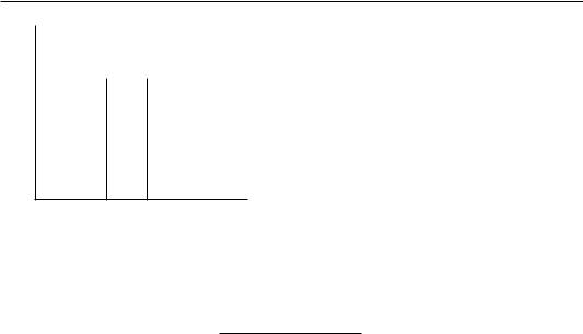
In Figure 2, we illustrate the effects on LAS and SAS that would result from an increase in full-employment GDP, due to an increase in labor, capital, or an advance in

technology. Long-run aggregate supply increases to LAS" and short-run aggregate supply increases to SAS 2 .

Figure 2: An Increase in Potential CDP

Price Level

p' _. -- - - - - -- -

SAS

1

Real Output (CDP)

There are some factors that will shift SAS, but not affect LAS. We held the money wage rate and other resource prices constant in constructing the SAS curve. If the wage rate or prices of other productive inputs increase, the SAS curve will shift to the left, a decrease

Study Session 5 Cross-Reference to CFA Institute Assigned Reading #23 - Aggregate Supply and Aggregate Demand

in short-run aggregate supply. When businesses observe a rise in resource prices, they will decrease their OUtput as the profit maximizing level of output declines.

Two important faCtors influence the change in money wage rates. One is unemployment; when unemployment rises, it puts downward pressure on the money wage rate as there

is an excess supply of labor at the current rate. Conversely, if the economy is temporarily operating above full-employment levels, there will be upward pressure on the money wage ratc. The second factor that can influence the money wage rate is inflation expectations. An expected increase in inflation will lead to increases in the money wage rate and an expected decrease in inflation will slow the increase of money wages.

LOS 23.b: Explain the components of and the factors that affect real GOP demanded, describe the aggregate demand curve and why it slopes downward, and explain the factors that can change aggregate demand.

\\'c' turn our a[(ention now to the aggregate demand curve. The agg.regatc demalld curVL' shlnn thc rel;\rion bl't\\"ccn the pricc kvcl ~lfld lhl' leal ljuall[i[\ o( hIlal go"d, ;lllci

,clvices (re31 CDP) demanded. The compOllC'I11S ofaggrcgatc demand are:

Consumption (el.

Invcstment 0).

Government spending (C l.

Net eXportS (X). which is ex pons minus imports.

3(Wre a ate demand = c: + I + C + X

t"lt"J ~

The aggregate demand curve is downward sloping (a good thing for a demand curve!) because at higher price levels, consumption, business investment, and exports will

all likely decrease. There are two effects here to consider. First, when the price level rises, individuals' real wealth decreases. Since they have less accumulated wealth in real terms, individuals will spend less. This is referred to as the "wealth effect," Second, when the price level increases. interesr rates will rise. An increase in interest rates decreases business investmenr (I) as well as consumption (C) as consumers delay or forego purchases of consumer durables such as cars, appliances and home repairs. This is a substitution effect, as consumers substitute consumption later for consumption now because the cost of consuming goods now instead of later (the interest rate) has increased. This is referred to as "inrertemporal substitution," substitution between time periods.

So changes in the price level cause changes in (the quantity of) aggregate demand. What factors will shift the aggregate uemand curve? Among the manr things that can affect aggregate demand there are three primary factors:

Expectations ahout future incomes, inflation, and profits.

Fiscal and monetary policy.

•World economy.

An increase in expected inflation will increase aggregate demand as consumers accelerate purchases to avoid higher prices in the future. An expectation of higher incomes in the future also will cause consumers to increase purchases in anticipation of these higher

Study Session 5

Cross-Reference to CFA Institute Assigned Reading #23 - Aggregate Supply and Aggregate Demand

incomes. An increase in expected profits will lead businesses to increase their investment in plant and equipment.

Fiscal policy refers to government policy with regard ro spending. taxes. and transfer payments. An increase in spending increases the government component (G) of aggregate demand. A decrease in taxes or an increase in transfer payments (e.g. social securiry benefirs or unemployment compensation) will increase the amount that consumers have to spend (their disposable income) and increase aggregate demand through an increase in consumption (C).

Monetary policy refers to the central bank's decisions to increase or decrease the money supply. An increase in the money supply will rend [0 decrease interest rates and increase consumption and investment spending. increasing aggregate demand. We will Jook at both monerary and fiscal policy effects more closely in subsequent topic reviews.

The srart; or rhe world econOI1l\ will inAuence a COllIHr:''s aggregare dem;1l1d rhrough the ncr exports (X) componellL. If foreign in~-omes increase. foreign demand for the LOUIHI"I', exports will increase. Increasing X. If rhe countI"l.'.,> foreign exchange rate increases (forL'ign currency bu\'s fewer' domestic CUITenC\' units). its goods are relarjveh' more expensive to foreigners, and exports will decrease. At the same time, imports wil I be relativel:· cheaper and the CJuanrir), of imporred goods demanded will increase. Both effects will tend to decrease net expons (expons minus imports. Xl and consequently' decrease aggregate demand. A decrease in a country's exchange rate (currency depreciation) will have the opposite effecr, increasing exports, decreasing imporrs. and increasing net exporrs and aggregate demand

LOS 23.c: Differentiate between short-run and long-run macroeconomic equilibrium, and explain how economic growth, inflation, and changes in aggregate demand and supply influence the macroeconomic equilibrium.

Now we examine macroeconomic equilibrium in the shorr run and in the long run.

In Figure 3. we illustrare long-run equilibrium ar the intersection of the LAS curve and the aggregate demand curve. Just as we saw that price was the variable that led us to equilibrium in the goods market in microeconomics, here changes in the price level of final goods and services can move the economy to long-run macroeconomic equilibrium. In Figure .3. equilibrium is at a price level of 110. If we are at a shorr-run disequilibrium with the price level at 115, there is excess supply; the quantity of real goods and services supplied exceeds the (aggregate) demand for real goods and services. This is sometimes termed a recessionarv gap. and there will be downward pressure on prices. Businesses will see a build-up of inventories and will decrease borh production and prices in response. This will result in a decrease in the price level. which will move rhe economy roward long-run equilibrium at a price level of 110. If the price level were 105. there would be excess demand for real goods and services. This is sometimes referred to as

an inflationary gap. Businesses will experience unintended decreases in inventories and respond by increasing output and prices. As the price level increases, the economy moves aJong the aggregate demand curve toward long-run equilibrium.

Study Session 5 - Cross-Reference to CFA Institute Assigned Reading #23 - Aggregate Supply and Aggregate Demand

Figure 3: Long-Run Equilibrium Real Output

!'rice l.evel (Index)

parr o( the proCeSS of moving toward rhL: IOllg-run equilibriul1l ourpul and flricc Iel'e!. Recall rhar in lonsrrucring rhe SAS curve WL: held mont'\' wages and orher resouru: prices consranr. Ie rhe econom:' is in shorr-run equilibrium, bur ar a level

ahove or helml full-emp!o\"lTIenr CDP, ir is in long-run disequilibrium. In Figure 4, we illusrrare rwo siruarions where rhe econorn:' is in shorr-run equilibrium bur nor in

long-run equilibrium. in panel (a). shorr-run Clluilibriu!1l real GOP, COP], is less rkllJ full employmenr GOP (along rhe LAS curve) and we would inrerprer rhis as J. recession or "below full-employment equilibrium." This difference berween real CDP and fuIlemployment GOP is called a recessionary gap or output gap. As we will derail, rhis brings downward pressure on money wages and resource prices rhal will decrease rhe equilibrium price level from P I to P·.

The opposire situarion, "above fuIl-employmenr equilibrium," is illusrrared in panel (b), where the shorr-run equilibrium real GOP' GOP l'is above the full-employment level. This would be rhe situarion in an economic expansion where aggregate demand has grown fas[er than LAS. The resulr will be upward pressure on prices rha[ will resulr in inflarion as rhe general price level increases from PI to P'.

Figure 4: Long-Run Dise<Juilibrium

Study Session 5

Cross-Reference to CFA Institute Assigned Reading #23 - Aggregate Supply ami Aggregate Demand

We have essentially described the phases of a business cycle here as deviations of shorrrun equilibrium real GOP below full-employment GOP (recession) and above fullemployment GOP (expansion leading to inflationary pressure). How does this happen? Changes in aggregate demand can drive these business cycles.

Consider the short-run and long-run adjustment to an increase in aggregate demand illustrated in Figure 5. From an initial state of long-run equilibrium at the intersection of ADo with LAS, assume that aggregate demand increases to AD l , The new shortrun equilibrium will be at over-full employment with real GOP, GOP I'above fullemployment GOP, GDP*. The increase in the price level (from Po to P SR) at the new

equilibrium level means that workers' real wages have decreased (we are holding money wages constant in the short run). At the same time, the increase in demand will cause businesses to attempt to increase produCtion, which will require hiring more worker~.

These two factors both lead to increased money wage demands. As these demands are met, we get a shift in the SAS curve from SAS o to SAS I'which will restore lonp:-run macroeconomic equilibriul11 at fll!l-el11plo~'meI1t real COP and al a ne\\" price k\'el

of P1lZ' ~ote Lhal an increase in the money wabc and other I"I'.rolll·(( prices mc:lllS thaI business \\"ill be' \\"illin b to sup)'h- less real good, and ,>en'ices at each price Ic\"cl I pri-:cs of final goods and ser\"iccs"l. Ir j, r11l'increase in resource prices that cameo SAS to decrease.

Figure 5: Adjustment to an Increase in Aggregate Demand

In Figure 6. we illustrate how a decrease in aggregate demand from ADo ro AD I will lead to a new short-run equilibrium with the price level at P SR and real GOP at GOP l'

GOP I is less than fuJJ-employment GOP (a recession). The resulting excess supply of labor (workers seeking jobs) will put downward pressure on money wage rates and other resource prices. This will lead ro a shifr in SAS to SAS j (an increase in supplyJ, restoring long-run equilibrium at full-employment GOP along the LAS curve and at a new, lower price level of I'u,'Remember, a decrease in wages and other input prices increases shorrrun aggregate supply.

LOS 2.1.d: Compare and contrast the classical, Keynesian, and monetarist schools or macroecunomics.

\X'hile our disclJ5sioJ1 of the forces leading (0 shorr-run and Ions-run macroeconomic equilibrium gives a basic description of business cycles and the forces that tend (() move the economy (Oward full employmem in the long run. there are differences of opinion on how well this process worb and the time lags between the shorr run and the long run.

The classical economists believed that shifts in both aggregate demand and aggregate supply were primarily driven bv changes in technology over time. Although classical economists did not use the aggregate supply-aggregate demand analysis we have presemed, their view of macroeconomic equilibrium is consistcnt with this analysis. We just need to add the assumption thar the long-run adjustmem of money wages ro restore full-employment equilibrium happens fairly rapidly and that rhe economy therefore

has a strong tendency (Oward full-employment equilibrium, as either recession or overfull employmenr lead to decreases or increases in the money wage rate. Their analysis concluded that taxes were the primary impediment (0 long-run equilibrium and that if the disrortions in inccmives from taxes were minimized, the economy would grow in an efficiem manner with increases in labor and capital and with improvements in technology.

The Great Depression of the 1930s did not suPPOrt the view of the classical economists. The economy in the U.S. operated significantly below itS full-employmem level

for many years. Additionally. business cycles in general were more severe and more prolonged than the classical model would suggest. John Maynard Kevnes was an economist who attempted (0 explain the depression and rhe nature of business cycles and ro provide policv recommendations for moving the economy toward full-employmem GOP and reducing rhe severity and duration of business cycles.

Keynes believed that shifts in aggregate demand due ro changes in expecrarions were the primary cause of business cycles and that wages were "downward sticky," reducing the ability of a decrease in money wages ro increase SAS and move the economy from recession (or depression) back towards the full-employment level of ourpUL The New Keynesians added (0 this model, asserting that the prices of Other productive inpurs

Study Session 5

Cross-Reference to CFA Institute Assigned Reading #23 - Aggregate Supply and Aggregate Demand

in addition ro labot ate also "downwatd sticky," ptesenting another barrier to the restoration of full-employment equilibrium.

The policy prescription of Keynesian economists was to direcdy increase aggregate demand through monetary policy (increasing the money supply) or through fiscal policy (increasing government spending, decreasing taxes, or both).

A third view of macroeconomic equilibrium is that held by monetarists. Monetarists believe that the main factor leading to business cycles and deviations from fullemployment equilibrium is monetary policy. They suggest that to keep aggregate demand stable and growing. the central bank should follow a policy of a steady and predictable increases in the money supply. Monetarists believe that recessions are caused by inappropriate decreases in the money supply and that recessions can be persistent because money wage rates are downward sticky (as do the Keynesiansl. Like the classical economists, however, they believe that the best tax policy is to keep taxes lo\\' to minimi/.e the disruption and distortion thar the\' introduce into the ,-,conOl11\" ar!d dlC resulting decrease in full-emplo\'rnenr CUP.

Study Session 5 Cross-Reference to CFA Institute Assigned Reading #23 - Aggregate Supply and Aggregate Demand

KEy CONCEPTS

LOS 23.a

Long-run aggregare supply is vertical at porential (full-employmenr) real GOP and can change as a resulr of changes in rhe labor force. rhe amount of capiral in rhe economy, or in technology.

Shorr-run aggregare supply is an increasing funcrion of rhe price level, is affecred by rhe same factors rhar affeer long-run aggregare supply, and is consrructed holding the money wage rare consrant. Money wages are assumed to depend directly on workers' expecrarions abour the furure rate of inRarion.

LOS 23.b

Aggregate demand is a decreasing function of the price level. Aggregate demand will increase with incrclses in incomes. a decrease in a counrr~:s exchange rare. or a rise in rhe expected ratt' of inflarion. Exp~lnsionalT11l0nnan' or fiscal polin' can both inLrClst' aggrq.:;alC demand.

From an initial long-run C(luilibriul1l. an increase (decrease) in aggregare demand will increa~e (decreastJ the price level and ourpul in [he shorr run. and the resultin~ increase (decrease) in money wages as workers' inflation expectations adjust to the new rate of inflcttion will decrease (increase) short-run aggregate supply, resulting in further price level increases (decreases) and a rerum to full-employmem long-run equilibrium.

LOS 2.~.d

The classical economists believed that rhe adjustment of money wages to restore fullemployment equilibrium is rapid and that without the distorting effecrs of taxes, long-run equilibrium real output would increase with increases in the labor force and accumulated capital, and with improvements in technology.

Keynesian economists believe that changes in expectations shifr aggregate demand, which causes business cycles, and that because wages are "downward sticky," the economy may not return rapidly from recession to fuJI-employment real GOP. Their policy prescription is to increase aggregate demand directly by expanding the money supplv or increasi ng the government defici t.

Monetarists believe that economic cycles are caused by inappropriate monetary policy and that a policy of stead~' and predictable increases in the monev supply, together with low taxes, willleJd to stahilit~· and maximum growth of real GOP.

Study Session 5

Cross-Reference to CFA Institute Assigned Reading #23 - Aggregate Supply and Aggregate Demand

CONCEPT CHECKERS

1. The economy's potential rate of output is best represented by:

A.long-run aggregate supply.

B.short-run aggregate supply. e. long-run aggregate demand.

2. Which of these factors is Least LikeLy to cause a shift in long-run aggregate supply?

A.Warfare destroys a large number of factories.

B.Prices of raw materials for production decrease.

e. An advance in technology increases the rate of productivity.

3.Aggregate demand is Least Like~y to include total:

A.net imports.

B.investment spending.

C. governmenr purchases.

"1. ';(ihich of the following boors would bt' leaST Iikl'/]' (0 shih rhe aggregate demand curvc~

A.The federal deficit expands.

B.Expected inflation decreases.

C.The price level increases.

5.1n shorr-run equilibrium, if aggregate demand is i ncreasi ng fasrt"f rhan long-run a:~~regate supply:

A.rhe price level is likely to increase.

C.downward pressure on wages should ensue.

e. supply will increase to meet the additional demand.

6.Which school of economic thought holds that unpredictable changes in central bank policy are the primary cause of business cycles?

A.Classical.

B.Keynesian. e. Monetarist.