диафрагмированные волноводные фильтры / 8f885481-2cf9-4d62-bb4f-fea568a0737a

P. Soto, A. Bergner, J.L. G´omez, V.E. Boria and H. Esteban

outlined at the beginning of Section 2.3. To illustrate this strategy, we next describe the optimization technique proposed for a uniform four-pole symmetric Chebyshev filter using the cavity lengths and the coupling window widths as design parameters (see Figure 2).

First, the ideal transfer function of the single first cavity (in a doubly terminated configuration) of the ideal network representation reported in Section 3.1 is computed. Next, the design parameters of the first cavity, the resonator length and the input and output aperture widths (see Figure 4), are tuned to recover the ideal response previously obtained. This task can be fully automated implementing the direct search and the gradient-based algorithm proposed in Section 2.3.

Output Waveguide

l1

Figure 4: Structure considered to tune the design parameters of the first cavity.

The next step considers the first two cavities (see Figure 5). Once the ideal response is obtained from the ideal network representation, the automated tuning procedure is repeated. This step only involves four physical parameters, namely, the additional cavity length and aperture width, and also the output aperture width and the resonator length of the previous cavity. These last two parameters must be slightly adjusted because of the interactions between adjacent cavities.

Figure 5: Structure considered to tune the design parameters of the first two cavities.

Then, we can add the remaining cavities to the filter with the same dimensions of

11

P. Soto, A. Bergner, J.L. G´omez, V.E. Boria and H. Esteban

the previous ones due to the symmetry of the structure. Finally, an additional optimization stage using only the BFGS gradient-based strategy on all the design parameters is performed.

According to the segmentation technique just described, any successive cavity always require the optimization of only four design parameters, thus improving both the robustness and e ciency of the whole optimization method.

A key feature in the multidimensional encapsulating algorithm is the order followed to optimize each individual physical parameter. As a general guideline, the new design parameters related to the added cavity must be always first tuned. Moreover, the cavity lengths are very critical parameters because they strongly a ect to the resonance frequency, so it is more convenient to tune them first.

The ideal responses of all the structures considered in the design procedure are only appropriate for moderate bandwidths, since the ideal network representations of such structures do not take into account the dispersive e ect of the real impedance inverters. Therefore, a suitable bandwidth must be chosen for each optimization stage, due to the impossibiliy of matching the ideal response on a large frequency range. The design experience recommends that all the optimization stages, excepting the last one, must only consider the pass band of the filter (slightly increased) to guarantee an excellent agreement. In order to improve the rejection response of the filter, the final optimization stage involving all the design parameters could also include the stop band of the filter.

3.3Design strategy of inductively coupled rectangular waveguide filters with tuning elements

The design procedure just explained before can be easily extended to the case of inductive filters including tuning elements. For these filters, the design parameters are the penetration depths of the tuning elements present in both the resonant cavities and the coupling windows (see Figure 3).

Unfortunately, these filters exhibit a strong mutual coupling between adjacent tuning elements. As a result, the decomposition technique must include an additional step before the final gradient-based optimization involving all the design parameters. Once the two parts of the filter are joined together, the penetration depths of the tuning elements placed in the central aperture and adjacent cavities must be adjusted to take into account their mutual coupling. This additional optimization stage requires the use of both the direct search method and the gradient-based algorithm previously described. Although not strictly necessary, it is convenient to also include in this new optimization step the input apertures of the two adjacent cavities.

4 APPLICATION EXAMPLES

The full-automated design procedure just proposed has been first applied to the design of two inductively coupled rectangular waveguide filters without tuning elements. The

12

P. Soto, A. Bergner, J.L. G´omez, V.E. Boria and H. Esteban

ideal transfer functions are standard four-pole Chebyshev responses of 300 MHz bandwidth and 0.02 dB ripple centered at 11 and 13 GHz, respectively.

The real waveguide structure proposed to design both filters is shown in Figure 2, where it can be seen that the cavity lengths and coupling aperture widths are chosen as design parameters. The input and output waveguides of the two filters, as well as the resonant cavities, are implemented with standard WR-75 waveguides (a = 19.050 mm, b = 9.525 mm). For all the coupling windows of both filters, the thickness value has been chosen equal to 2.00 mm.

The precise simulation tool used in the VS required a total number of 25 modes to obtain the GAM representation of each building block of the structure, and 6 modes for assembling the final system (the so called localized and accesible modes [25], respectively). The fast coarse model in the OS only considers the first 2 modal solutions for both the accessible and localized modes.

For the two filters under consideration, the staring points required by the initial optimizations in the OS have been determined according to the method proposed in Section 3.1. A summary of the parameter values of such starting points (x(0)os ) is o ered in Table 1. For both filters, the decomposition technique described in Section 3.2 has been followed to perform the first parameter extraction in the OS leading to xos (see values in Table 1).

Table 1: Values of the design parameters for the two inductive filters without tuning elements.

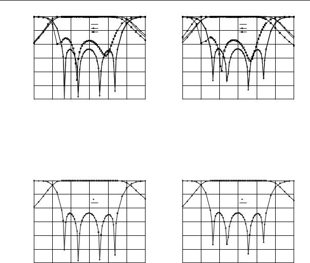
The electrical responses of both filters obtained using the coarse and fine models at xos are compared in Figure 6 with the corresponding ideal objective function. As expected, a very good agreement between the ideal response and the one obtained with the coarse model is concluded in both cases, whereas a certain disagreement can be observed between the coarse and fine model responses.

With regard to the remaining parameter extraction phases of the ASM design technique, they were accomplished acting on all the design parameters at the same time, because of the high similarity between the responses obtained in the VS and in the OS. The complete ASM design procedure only required 3 iterations to converge. For comparative reasons, the values of the design parameters for the final ASM solution in the validation space xem are compiled in Table 1.

13

P. Soto, A. Bergner, J.L. G´omez, V.E. Boria and H. Esteban

Figure 6: Responses of filters (no tuning) using the coarse and fine models at xos and ideal functions.

In Figure 7, a comparison between the scattering parameters obtained with the fine simulation tool at xem and the results obtained with the coarse model at xos is shown. It is concluded that the desired objective function has been finally recovered in the VS.

Figure 7: Responses of filters (no tuning) using the coarse model at xos and the fine model at xem.

Starting from the same initial points, the two inductive filters were also designed using directly the precise simulation tool and the segmentation technique described in Section 3.2. A comparative study in terms of the CPU time required by the ASM technique and the direct optimization procedure is reported in Table 2. The results reveal that the design procedure based on the ASM technique is about 10 times faster.

Table 2: CPU time (Pentium III 450 MHz PC) required to design the two inductive filters (no tuning).

14

P. Soto, A. Bergner, J.L. G´omez, V.E. Boria and H. Esteban

Table 3: Dimensions of the cavities and coupling windows for the common inductive geometry of the two filters with tuning elements.

Finally, two more complex inductively coupled rectangular waveguide filters with tuning elements (see Figure 3) were designed to recover the same previous ideal responses. As can be seen in Figure 3, the design parameters for both filters are the penetration depths of the tuning elements placed at the cavities and coupling apertures. With regard to the other dimensions of the structures considered, they were deduced from the inductive filter without tuning elements previously designed at 13 GHz, but reducing the coupling window widths and the cavities lengths in order to be able to recover the two desired responses using tuning elements [12]. The values of such physical parameters are therefore the same for both filters, and can be seen in Table 3.

For these cases, the fine EM simulator required a total number of 90 localized modes and 30 accessible modes. The fast coarse model only needed the first 10 modal solutions for both the accessible and localized modes.

The ASM starting point x(0)os for the two filters with tuning elements under study were obtained according to the method detailed in Section 3.1. The decomposition technique proposed in Section 3.3 was then applied to accomplish the first parameter extraction in the OS, which determines the coarse solution xos. The tuning element penetration depths at x(0)os and xos for both filters are compiled in Table 4.

Table 4: Values of the design parameters for the two inductive filters with tuning elements.

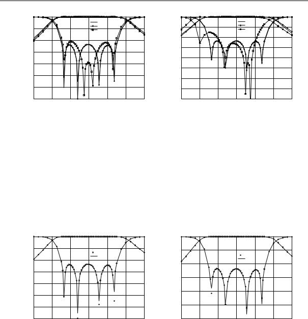
In Figure 8, the S-parameters of both filters obtained using the coarse and fine models at xos are compared with the corresponding ideal objective response. It can be observed that the ideal response and the one obtained with the coarse model are quite similar. On the contrary, the coarse and fine model responses are severely misaligned.

15

P. Soto, A. Bergner, J.L. G´omez, V.E. Boria and H. Esteban

Figure 8: Responses of both filters (with tuning) using the coarse and fine models at xos and ideal objective functions.

In this case, the remaining parameter extraction phases must be performed using the same segmentation procedure employed with the initial optimization, because the VS and OS responses are not similar enough. Nevertheless, the complete ASM design procedure only required 3 iterations to reach convergence. The values of the design parameters for the final ASM solution in the VS (xem) can be found in Table 4.

A comparison between the scattering parameters for both filters computed with the fine model at xem and with the coarse EM simulator at xos is o ered in Figure 9. These results reveal that the desired objective functions have been finally reproduced in the VS.

Figure 9: Responses of both filters (with tuning) using the coarse model at xos and the fine model at

xem.

The ASM design procedure of filters with tuning elements centered at 11 and 13 GHz required a total CPU time of 903 min. and 647 min., respectively, on a Pentium III 450 MHz PC. These CPU times would have been highly increased if a direct optimization procedure had been employed.

16

P. Soto, A. Bergner, J.L. G´omez, V.E. Boria and H. Esteban

5 CONCLUSIONS

In this paper, the ASM procedure is successfully applied to the full-automated design of inductive rectangular waveguide filters. For both the coarse and fine model of the ASM technique, the same modal analysis tool based on the GAM representation is proposed. To control the accuracy and e ciency of each model, the number of modes in the multimode network representations of the structures considered has been suitably chosen. For the parameter extraction phases of the ASM technique, which are the most CPU time consuming stages of such design procedure, a combined strategy using a new multidimensional direct search algorithm and a gradient-based method is fully described. With the aim of improving the robustness and e ciency of such strategy, a classical segmentation design technique is properly revisited. In order to increase the e ciency of the first parameter extraction required in the OS space, a novel procedure to determine a good starting point is also proposed. To validate the new design procedure presented, two inductively coupled rectangular waveguide filters without tuning elements have been first designed. Next, the same electrical responses have also been recovered using more complex structures including tuning elements. CPU comparative studies for such cases have also been included, thus revealing the e ciency of the new design strategy outlined. As future research line, the authors propose to use the ASM design procedure with other waveguide structures of interest in the telecommunication sector.

ACKNOWLEDGEMENTS

This work has been supported in part by Conselleria de Cultura, Educaci´on y Ciencia, Generalitat Valenciana, under Research Project Ref. GV98-14-68, and in part by a Research Funding Programme of Universidad Polit´ecnica de Valencia.

Contract grant sponsor of Mr. P. Soto (Ref. AP99 23003909): Ministerio de Educaci´on y Ciencia, Spain.

17

P. Soto, A. Bergner, J.L. G´omez, V.E. Boria and H. Esteban

REFERENCES

[1]J.W. Bandler (Editor), Special Issue on “Automated circuit design using electromagnetic simulators”, IEEE Trans. Microwave Theory Tech., 45, part II, 709-866 (1997).

[2]F. Alessandri, M. Dionigi and R. Sorrentino, “A fullwave CAD tool for waveguide components using a high speed direct optimizer”, IEEE Trans. Microwave Theory Tech., 43, 2046-2052 (1995).

[3]M. Guglielmi, “Simple CAD procedure for microwave filters and multiplexers”, IEEE Trans. Microwave Theory Tech., 42, 1347-1352 (1994).

[4]J.T. Alos and M. Guglielmi, “Simple and e ective EM-based optimization procedure for microwave filters”, IEEE Trans. Microwave Theory Tech., 45, 856-858 (1997).

[5]J.W. Bandler, R.M. Biernacki, S.H. Chen, P.A. Grobelny and R.H. Hemmers, “Space mapping technique for electromagnetic optimization”, IEEE Trans. Microwave Theory Tech., 42, 2536-2544 (1994).

[6]J.W. Bandler, R.M. Biernacki, S.H. Chen, R.H. Hemmers and K. Madsen, “Electromagnetic optimization exploiting aggressive space mapping”, IEEE Trans. Microwave Theory Tech., 43, 2874-2881 (1995).

[7]J.W. Bandler, R.M. Biernacki, S.H. Chen and Y.F. Huang, “Design optimization of interdigital filters using aggressive space mapping and decomposition”, IEEE Trans. Microwave Theory Tech., 45, 761-769 (1997).

[8]J.W. Bandler, R.M. Biernacki, S.H. Chen, L.W. Hendrick and D. Omeragi´c, “Electromagnetic optimization of 3-D structures”, IEEE Trans. Microwave Theory Tech., 45, 770-779 (1997).

[9]J.W. Bandler, R.M. Biernacki, S.H. Chen and D. Omeragi´c, “Space mapping optimization of waveguide filters using finite elements and mode-matching electromagnetic simulators”, in IEEE MTT-S Int. Microwave Symp. Dig., Denver, CO, 635-638 (1997).

[10]A. Alvarez, G. Connor and M. Guglielmi, “New simple procedure for the computation of the multimode admittance or impedance matrix of planar waveguide junctions”,

IEEE Trans. Microwave Theory Tech., 44, 413-418 (1996).

[11]C. Kudsia, R. Cameron and W.-C. Tang, “Innovations in microwave filters and multiplexing networks for communications satellite systems”, IEEE Trans. Microwave Theory Tech., 40, 1133-1194 (1992).

18

P.Soto, A. Bergner, J.L. G´omez, V.E. Boria and H. Esteban

[12]V.E. Boria, M. Guglielmi and P. Arcioni, “Computer-aided design of inductively coupled rectangular waveguide filters including tuning elements”, Int. Journal of RF and Microwave Computer-Aided Engineering, 8, 226-235 (1998).

[13]G. Conciauro, M. Guglielmi and R. Sorrentino, Advanced modal analysis - CAD techniques for waveguide components and filters, John Wiley & Sons Ltd., 2000.

[14]C.G. Broyden, “A class of methods for solving nonlinear simultaneous equations”, Math. Comp., 19, 577-593 (1965).

[15]V.E. Boria and M. Guglielmi, “Accelerated computation of admittance parameters for planar waveguide junctions”, Int. Journal of Microw. and Millimeter-Wave Computer-Aided Engineering, 7, 195-205 (1997).

[16]G. Conciauro, M. Bressan and C. Zu ada, “Waveguide modes via an integral equation leading to a linear matrix eigenvalue problem”, IEEE Trans. on Microw. Theory Tech., 32, 1495-1504 (1984).

[17]P Arcioni, “Fast evaluation of modal coupling coe cients of waveguide step discontinuities”, IEEE Microw. and Guided Wave Lett., 6, 232-234 (1996).

[18]R.E. Collin, Foundations for microwave engineering, McGraw Hill, 1992.

[19]V.E. Boria, G. Gerini and M. Guglielmi, “An e cient inversion technique for banded linear systems”, in IEEE MTT-S Int. Microwave Symp. Dig., Denver, CO, 1567-1570 (1997).

[20]J.W. Bandler, “Optimization methods for computer-aided design”, IEEE Trans. Microwave Theory Tech., 17, 533-552 (1969).

[21]H.H. Rosenbrock, “An automatic method for finding the greatest or least value of a function”, Computer J., 3, 175-184 (1960).

[22]W.H. Press, S.A. Teukolsky, W.T. Vetterling and B.P. Flannery, Numerical recipes in fortran 77: The art of scientific computing, Cambridge University Press, 1992.

[23]G. Matthaei, L. Young and E.M.T. Jones, Microwave filters, impedance-matching networks, and coupling structures, Artech House Inc., 1980.

[24]N. Marcuvitz, Waveguide handbook, Peter Peregrinus Ltd., 1993.

[25]T. Rozzi and M. Mongiardo, “E-plane steps in rectangular waveguide”, IEEE Trans. on Microw. Theory Tech., 39, 1279-1288 (1991).

19